spectractor.extractor package

Submodules

spectractor.extractor.chromaticpsf module

class spectractor.extractor.chromaticpsf.ChromaticPSF(psf, Nx, Ny, x0=0, y0=None, deg=4, saturation=None, file_name='')[source]

Bases: object

Class to store a PSF evolving with wavelength.

The wavelength evolution is stored in an Astropy table instance. Whatever the PSF model, the common keywords are:

lambdas: the wavelength [nm]
Dx: the distance along X axis to order 0 position of the PSF model centroid [pixels]
Dy: the distance along Y axis to order 0 position of the PSF model centroid [pixels]
Dy_disp_axis: the distance along Y axis to order 0 position of the mean dispersion axis [pixels]
flux_sum: the transverse sum of the data flux [spectrogram units]
flux_integral: the integral of the best fitting PSF model to the data (should be equal to the amplitude parameter

of the PSF model if the model is correclty normalized to one) [spectrogram units] * flux_err: the uncertainty on flux_sum [spectrogram units] * fwhm: the FWHM of the best fitting PSF model [pixels] * Dy_fwhm_sup: the distance along Y axis to order 0 position of the upper FWHM edge [pixels] * Dy_fwhm_inf: the distance along Y axis to order 0 position of the lower FWHM edge [pixels]

Then all the specific parameter of the PSF model are stored in other columns with their wavelength evolution (read from PSF.param_names attribute).

A saturation level should be specified in data units.

build_psf_cube(pixels, profile_params, fwhmx_clip=2, fwhmy_clip=2, dtype='float64', mask=None, boundaries=None)[source]

Build a cube, with one slice per wavelength evaluation which contains the PSF evaluation.

Parameters:

pixels (np.ndarray) – Array of pixels to evaluate ChromaticPSF.
profile_params (array_like) – ChromaticPSF profile parameters.
fwhmx_clip (int, optional) – Clip PSF evaluation outside fwhmx*FWHM along x axis (default: parameters.PSF_FWHM_CLIP).
fwhmy_clip (int, optional) – Clip PSF evaluation outside fwhmy*FWHM along y axis (default: parameters.PSF_FWHM_CLIP).
dtype (str, optional) – Type of the output array (default: ‘float64’).
mask (array_like, optional) – Cube of booleans where values are masked (default: None).
boundaries (dict, optional) – Dictionary of boundaries for fast evaluation with keys ymin, ymax, xmin, xmax (default: None).

Returns:

psf_cube – Cube of chromatic PSF evaluations, each slice being a PSF for a given wavelength.

Return type:

np.ndarray

Examples

>>> s = ChromaticPSF(Moffat(), Nx=100, Ny=20, deg=2, saturation=20000)
>>> profile_params = s.from_poly_params_to_profile_params(s.generate_test_poly_params(), apply_bounds=True)
>>> profile_params[:, 1] = np.arange(s.Nx)
>>> psf_cube = s.build_psf_cube(s.set_pixels(mode="2D"), profile_params)
>>> psf_cube.shape
(100, 20, 100)
>>> plt.imshow(psf_cube[20], origin="lower"); plt.show()  
<matplotlib.image.AxesImage object at ...>
>>> plt.imshow(psf_cube[80], origin="lower"); plt.show()  
<matplotlib.image.AxesImage object at ...>

build_psf_cube_masked(pixels, profile_params, fwhmx_clip=2, fwhmy_clip=2)[source]

Build a boolean cube, with one slice per wavelength evaluation which contains booleans where PSF evaluation is non zero.

Parameters:

pixels (np.ndarray) – Array of pixels to evaluate ChromaticPSF.
profile_params (array_like) – ChromaticPSF profile parameters.
fwhmx_clip (int, optional) – Clip PSF evaluation outside fwhmx*FWHM along x axis (default: parameters.PSF_FWHM_CLIP).
fwhmy_clip (int, optional) – Clip PSF evaluation outside fwhmy*FWHM along y axis (default: parameters.PSF_FWHM_CLIP).

Returns:

psf_cube_masked – Cube of chromatic masked PSF evaluations, each slice being a PSF for a given wavelength.

Return type:

np.ndarray

Examples

>>> s = ChromaticPSF(Moffat(), Nx=100, Ny=20, deg=2, saturation=20000)
>>> profile_params = s.from_poly_params_to_profile_params(s.generate_test_poly_params(), apply_bounds=True)
>>> profile_params[:, 1] = np.arange(s.Nx)
>>> psf_cube_masked = s.build_psf_cube_masked(s.set_pixels(mode="2D"), profile_params)
>>> psf_cube_masked.shape
(100, 20, 100)
>>> plt.imshow(psf_cube_masked[20], origin="lower"); plt.show()  
<matplotlib.image.AxesImage object at ...>
>>> plt.imshow(psf_cube_masked[80], origin="lower"); plt.show()  
<matplotlib.image.AxesImage object at ...>

build_psf_jacobian(pixels, profile_params, psf_cube_sparse_indices, boundaries, dtype='float32')[source]

Compute the Jacobian matrix \(\mathbf{J}\) of a ChromaticPSF model, with analytical derivatives. Amplitude parameters \(\mathbf{A}\) are excluded, only PSF shape and position parameters \(\theta\) are included.

\[\mathbf{J} = \frac{\partial \mathbf{M}}{\partial \theta} \cdot \mathbf{A}.\]

Parameters:

pixels (np.ndarray) – Array of pixels to evaluate ChromaticPSF.
profile_params (array_like) – ChromaticPSF profile parameters.
psf_cube_sparse_indices (array_like) – Array of indices where each element gives the sparse indices for a slice of the ChromaticPSF cube.
boundaries (dict) – Dictionary of boundaries for fast evaluation with keys ymin, ymax, xmin, xmax .
dtype (str, optional) – Type of the output array (default: ‘float32’).

Returns:

J – The Jacobian matrix math:mathbf{J}.

Return type:

np.ndarray

Examples

>>> s = ChromaticPSF(Moffat(), Nx=100, Ny=20, deg=2, saturation=20000)
>>> profile_params = s.from_poly_params_to_profile_params(s.generate_test_poly_params(), apply_bounds=True)
>>> profile_params[:, 0] = np.ones(s.Nx)  # normalized PSF
>>> profile_params[:, 1] = np.arange(s.Nx)  # PSF x_c positions
>>> psf_cube_masked = s.build_psf_cube_masked(s.set_pixels(mode="2D"), profile_params)
>>> psf_cube_masked = s.convolve_psf_cube_masked(psf_cube_masked)
>>> boundaries, psf_cube_masked = s.set_rectangular_boundaries(psf_cube_masked)
>>> psf_cube_sparse_indices, M_sparse_indices = s.get_sparse_indices(boundaries)
>>> s.params.fixed[s.Nx:s.Nx+s.deg+1] = [True] * (s.deg+1)  # fix all x_c parameters
>>> J = s.build_psf_jacobian(s.set_pixels(mode="2D"), profile_params, psf_cube_sparse_indices, boundaries, dtype="float32")
>>> J.shape
(13, 2000)
>>> J.dtype
dtype('float32')
>>> plt.imshow(J[s.params.get_index("y_c_0")-s.Nx].reshape((s.Ny, s.Nx)), origin="lower"); plt.show()  
<matplotlib.image.AxesImage object at ...>

build_sparse_M(pixels, profile_params, M_sparse_indices, boundaries, dtype='float32')[source]

Compute the sparse model matrix \(\mathbf{M}\). Given a vector of amplitudes \(\mathbf{A}\), spectrogram model is: .. math:

\mathbf{I} = \mathbf{M} \cdot \mathbf{A}.

Parameters:

pixels (np.ndarray) – Array of pixels to evaluate ChromaticPSF.
profile_params (array_like) – ChromaticPSF profile parameters.
M_sparse_indices (array_like) – Array of indices where each element gives the sparse indices for a slice of the ChromaticPSF cube.
boundaries (dict) – Dictionary of boundaries for fast evaluation with keys ymin, ymax, xmin, xmax .
dtype (str, optional) – Type of the output array (default: ‘float32’).

Returns:

M – The model matrix \(\mathbf{M}\).

Return type:

np.ndarray

Examples

>>> s = ChromaticPSF(Moffat(), Nx=100, Ny=20, deg=2, saturation=20000)
>>> profile_params = s.from_poly_params_to_profile_params(s.generate_test_poly_params(), apply_bounds=True)
>>> profile_params[:, 0] = np.ones(s.Nx)  # normalized PSF
>>> profile_params[:, 1] = np.arange(s.Nx)  # PSF x_c positions

2D case

>>> psf_cube_masked = s.build_psf_cube_masked(s.set_pixels(mode="2D"), profile_params)
>>> psf_cube_masked = s.convolve_psf_cube_masked(psf_cube_masked)
>>> boundaries, psf_cube_masked = s.set_rectangular_boundaries(psf_cube_masked)
>>> psf_cube_sparse_indices, M_sparse_indices = s.get_sparse_indices(boundaries)
>>> M = s.build_sparse_M(s.set_pixels(mode="2D"), profile_params, M_sparse_indices, boundaries, dtype="float32")
>>> M.shape
(2000, 100)
>>> M.dtype
dtype('float32')
>>> plt.imshow((M @ np.ones(s.Nx)).reshape((s.Ny, s.Nx)), origin="lower"); plt.show()  
<matplotlib.image.AxesImage object at ...>

1D case

>>> psf_cube_masked = s.build_psf_cube_masked(s.set_pixels(mode="1D"), profile_params)
>>> psf_cube_masked = s.convolve_psf_cube_masked(psf_cube_masked)
>>> boundaries, psf_cube_masked = s.set_rectangular_boundaries(psf_cube_masked)
>>> psf_cube_sparse_indices, M_sparse_indices = s.get_sparse_indices(boundaries)
>>> M = s.build_sparse_M(s.set_pixels(mode="1D"), profile_params, M_sparse_indices, boundaries, dtype="float32")
>>> M.shape
(2000, 100)
>>> M.dtype
dtype('float32')
>>> plt.imshow((M @ np.ones(s.Nx)).reshape((s.Ny, s.Nx)), origin="lower"); plt.show()  
<matplotlib.image.AxesImage object at ...>

build_sparse_dM(pixels, profile_params, M_sparse_indices, boundaries, dtype='float32')[source]

Compute the partial derivatives of the model matrix \(\mathbf{M}\), with analytical derivatives. Amplitude parameters \(\mathbf{A}\) are excluded, only PSF shape and position parameters \(\theta\) are included.

Parameters:

pixels (np.ndarray) – Array of pixels to evaluate ChromaticPSF.
profile_params (array_like) – ChromaticPSF profile parameters.
M_sparse_indices (array_like) – Sparse indices of the model matrix \(\mathbf{M}\).
boundaries (dict) – Dictionary of boundaries for fast evaluation with keys ymin, ymax, xmin, xmax .
dtype (str, optional) – Type of the output array (default: ‘float32’).

Returns:

dM – List of sparse matrices \(\partial \mathbf{M}/\partial \theta\)

Return type:

list

Examples

>>> s = ChromaticPSF(Moffat(), Nx=100, Ny=20, deg=2, saturation=20000)
>>> profile_params = s.from_poly_params_to_profile_params(s.generate_test_poly_params(), apply_bounds=True)
>>> profile_params[:, 0] = np.ones(s.Nx)  # normalized PSF
>>> profile_params[:, 1] = np.arange(s.Nx)  # PSF x_c positions
>>> psf_cube_masked = s.build_psf_cube_masked(s.set_pixels(mode="2D"), profile_params)
>>> psf_cube_masked = s.convolve_psf_cube_masked(psf_cube_masked)
>>> boundaries, psf_cube_masked = s.set_rectangular_boundaries(psf_cube_masked)
>>> psf_cube_sparse_indices, M_sparse_indices = s.get_sparse_indices(boundaries)
>>> s.params.fixed[s.Nx:s.Nx+s.deg+1] = [True] * (s.deg+1)  # fix all x_c parameters
>>> dM = s.build_sparse_dM(s.set_pixels(mode="2D"), profile_params, M_sparse_indices, boundaries, dtype="float32")
>>> len(dM), dM[0].shape
(13, (2000, 100))
>>> dM[0].dtype
dtype('float32')
>>> plt.imshow((dM[s.params.get_index("y_c_0")-s.Nx] @ np.ones(s.Nx)).reshape((s.Ny, s.Nx)), origin="lower"); plt.show()  
<matplotlib.image.AxesImage object at ...>

static convolve_psf_cube_masked(psf_cube_masked)[source]

Convolve the ChromaticPSF cube of boolean values to enlarge a bit the mask.

Parameters:: psf_cube_masked (np.ndarray) – A ChromaticPSF cube.
Returns:: psf_cube_masked – Cube of boolean values where psf_cube cube is positive, eventually convolved.
Return type:: np.ndarray

Examples

>>> s = ChromaticPSF(Moffat(), Nx=100, Ny=20, deg=2, saturation=20000)
>>> profile_params = s.from_poly_params_to_profile_params(s.generate_test_poly_params(), apply_bounds=True)
>>> profile_params[:, 1] = np.arange(s.Nx)
>>> psf_cube_masked = s.build_psf_cube_masked(s.set_pixels(mode="2D"), profile_params)
>>> psf_cube_masked = s.convolve_psf_cube_masked(psf_cube_masked)
>>> psf_cube_masked.dtype
dtype('bool')
>>> psf_cube_masked.shape
(100, 20, 100)
>>> plt.imshow(psf_cube_masked[20], origin="lower"); plt.show()  
<matplotlib.image.AxesImage object at ...>
>>> plt.imshow(psf_cube_masked[80], origin="lower"); plt.show()  
<matplotlib.image.AxesImage object at ...>

crop_table(new_Nx)[source]

Crop the table to a new length size.

Parameters:: new_Nx (int) – New length of the ChromaticPSF on X axis.

Examples

>>> psf = Moffat()
>>> s = ChromaticPSF(psf, Nx=20, Ny=5, deg=1, saturation=20000)
>>> params = s.generate_test_poly_params()
>>> s.fill_table_with_profile_params(s.from_poly_params_to_profile_params(params))
>>> print(np.sum(s.table["gamma"]))
100.0
>>> print(s.table["gamma"].size)
20
>>> s.crop_table(10)
>>> print(np.sum(s.table["gamma"]))
50.0
>>> print(s.table["gamma"].size)
10

evaluate(pixels, poly_params, fwhmx_clip=2, fwhmy_clip=2, dtype='float64', mask=None, boundaries=None)[source]

Simulate a 2D spectrogram of size Nx times Ny.

Given a set of polynomial parameters defining the chromatic PSF model, a 2D spectrogram is produced either summing transverse 1D PSF profiles along the dispersion axis, or full 2D PSF profiles.

Parameters:

pixels (array_like) – The pixel array. If pixels.ndim==1, ChromaticPSF is evaluated using 1D PSF slices. Otherwise, pixels must have a shape like (2, Nx, Ny).
poly_params (array_like) – Parameter array of the model, in the form: - Nx first parameters are amplitudes for the Moffat transverse profiles - next parameters are polynomial coefficients for all the PSF parameters in the same order as in PSF definition, except amplitude.
fwhmx_clip (int, optional) – Clip PSF evaluation outside fwhmx*FWHM along x axis (default: parameters.PSF_FWHM_CLIP).
fwhmy_clip (int, optional) – Clip PSF evaluation outside fwhmy*FWHM along y axis (default: parameters.PSF_FWHM_CLIP).
dtype (str, optional) – Type of the output array (default: ‘float64’).
mask (array_like, optional) – Cube of booleans where values are masked (default: None).
boundaries (dict, optional) – Dictionary of boundaries for fast evaluation with keys ymin, ymax, xmin, xmax (default: None).

Returns:

output – A 2D array with the model.

Return type:

array

Examples

>>> psf = MoffatGauss()
>>> s = ChromaticPSF(psf, Nx=100, Ny=20, deg=4, saturation=20000)
>>> poly_params = s.generate_test_poly_params()

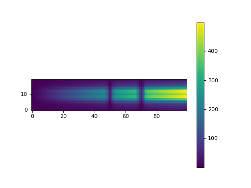
1D evaluation:

>>> output = s.evaluate(s.set_pixels(mode="1D"), poly_params)
>>> im = plt.imshow(output, origin='lower')  
>>> plt.colorbar(im)  
<matplotlib.colorbar.Colorbar object at 0x...>
>>> plt.show()

(Source code)

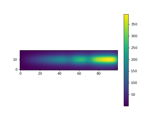
2D evaluation:

>>> output = s.evaluate(s.set_pixels(mode="2D"), poly_params)
>>> im = plt.imshow(output, origin='lower')  
>>> plt.colorbar(im)  
<matplotlib.colorbar.Colorbar object at 0x...>
>>> plt.show()

(Source code)

fill_table_with_profile_params(profile_params)[source]

Fill the table with the profile parameters.

Parameters:: profile_params (np.ndarray) – a Nx * len(self.psf.param_names) numpy array containing the PSF parameters as a function of pixels.

Examples

>>> psf = MoffatGauss()
>>> s = ChromaticPSF(psf, Nx=100, Ny=100, deg=4, saturation=8000)
>>> poly_params_test = s.generate_test_poly_params()
>>> profile_params = s.from_poly_params_to_profile_params(poly_params_test)
>>> s.fill_table_with_profile_params(profile_params)

fit_chromatic_psf(data, mask=None, bgd_model_func=None, data_errors=None, mode='1D', analytical=True, amplitude_priors_method='noprior', verbose=False, live_fit=False)[source]

Fit a chromatic PSF model on 2D data.

Parameters:

data (np.array) – 2D array containing the image data.
mask (np.array, optional) – 2D array containing the masked pixels.
bgd_model_func (callable, optional) – A 2D function to model the extracted background (default: None -> null background)
data_errors (np.array) – the 2D array uncertainties.
mode (str, optional) – Set the fitting mode: either transverse 1D PSF profile (mode=”1D”) or full 2D PSF profile (mode=”2D”).
amplitude_priors_method (str, optional) – Prior method to use to constrain the amplitude parameters of the PSF (default: “noprior”).
verbose (bool, optional) – Set the verbosity of the fitting process (default: False).

Returns:

w – The ChromaticPSFFitWorkspace containing info abut the fitting process.

Return type:

ChromaticPSFFitWorkspace

Examples

Set the parameters:

>>> parameters.PIXDIST_BACKGROUND = 40
>>> parameters.PIXWIDTH_BACKGROUND = 10
>>> parameters.PIXWIDTH_SIGNAL = 30
>>> parameters.DEBUG = True

Build a mock spectrogram with random Poisson noise using the full 2D PSF model:

>>> psf = Moffat(clip=False)
>>> s0 = ChromaticPSF(psf, Nx=120, Ny=100, deg=2, saturation=10000000)
>>> params = s0.generate_test_poly_params()
>>> params[:s0.Nx] *= 1
>>> s0.params.values = params
>>> saturation = params[-1]
>>> data = s0.evaluate(s0.set_pixels(mode="2D"), params)
>>> bgd = 10*np.ones_like(data)
>>> data += bgd
>>> data = np.random.poisson(data)
>>> data_errors = np.sqrt(np.abs(data+1))
>>> mask = np.zeros_like(data).astype(bool)
>>> mask[10:30,20:22] = True

Extract the background:

>>> bgd_model_func, _, _ = extract_spectrogram_background_sextractor(data, data_errors, ws=[30,50])

Propagate background uncertainties:

>>> data_errors = np.sqrt(data_errors**2 + bgd_model_func(np.arange(s0.Nx), np.arange(s0.Ny)))

Estimate the first guess values:

>>> s = ChromaticPSF(psf, Nx=120, Ny=100, deg=2, saturation=saturation)
>>> s.fit_transverse_PSF1D_profile(data, data_errors, w=20, ws=[30,50],
... pixel_step=1, bgd_model_func=bgd_model_func, saturation=saturation, live_fit=False)
>>> s.plot_summary(truth=s0)
>>> amplitude_residuals = [ [s0.params.values[:s0.Nx], np.array(s.table["amplitude"])-s0.params.values[:s0.Nx],
... np.array(s.table['amplitude'] * s.table['flux_err'] / s.table['flux_sum'])] ]

Fit the data using the transverse 1D PSF model only:

>>> w = s.fit_chromatic_psf(data, mode="1D", data_errors=data_errors, bgd_model_func=bgd_model_func,
... amplitude_priors_method="noprior", verbose=True, mask=mask)
>>> s.plot_summary(truth=s0)
>>> amplitude_residuals.append([s0.params.values[:s0.Nx], w.amplitude_params-s0.params.values[:s0.Nx],
... w.amplitude_params_err])

Fit the data using the full 2D PSF model

>>> parameters.PSF_FIT_REG_PARAM = 0.002
>>> w = s.fit_chromatic_psf(data, mode="2D", data_errors=data_errors, bgd_model_func=bgd_model_func,
... amplitude_priors_method="psf1d", verbose=True, analytical=True, mask=mask)
>>> s.plot_summary(truth=s0)
>>> amplitude_residuals.append([s0.params.values[:s0.Nx], w.amplitude_params-s0.params.values[:s0.Nx],
... w.amplitude_params_err])
>>> for k, label in enumerate(["Transverse", "PSF1D", "PSF2D"]):
...     plt.errorbar(np.arange(s0.Nx), amplitude_residuals[k][1]/amplitude_residuals[k][2],
...                  yerr=amplitude_residuals[k][2]/amplitude_residuals[k][2],
...                  fmt="+", label=label)  
<ErrorbarContainer ...>
>>> plt.grid()
>>> plt.legend()  
<matplotlib.legend.Legend object at ...>
>>> plt.show()

fit_transverse_PSF1D_profile(data, err, w, ws, pixel_step=1, bgd_model_func=None, saturation=None, live_fit=False, sigma_clip=5)[source]

Fit the transverse profile of a 2D data image with a PSF profile. Loop is done on the x-axis direction. An order 1 polynomial function is fitted to subtract the background for each pixel with a 3*sigma outlier removal procedure to remove background stars.

Parameters:

data (array) – The 2D array image. The transverse profile is fitted on the y direction for all pixels along the x direction.
err (array) – The uncertainties related to the data array.
w (int) – Half width of central region where the spectrum is extracted and summed (default: 10)
ws (list) – up/down region extension where the sky background is estimated with format [int, int] (default: [20,30])
pixel_step (int, optional) – The step in pixels between the slices to be fitted (default: 1). The values for the skipped pixels are interpolated with splines from the fitted parameters.
bgd_model_func (callable, optional) – A 2D function to model the extracted background (default: None -> null background)
saturation (float, optional) – The saturation level of the image. Default is set to twice the maximum of the data array and has no effect.
live_fit (bool, optional) – If True, the transverse profile fit is plotted in live accross the loop (default: False).
sigma_clip (int) – Sigma for outlier rejection (default: 5).

Examples

Build a mock spectrogram with random Poisson noise:

>>> psf = MoffatGauss()
>>> s0 = ChromaticPSF(psf, Nx=100, Ny=100, saturation=1000)
>>> s0.params.values = s0.generate_test_poly_params()
>>> saturation = s0.params.values[-1]
>>> data = s0.evaluate(s0.set_pixels(mode="1D"), s0.params.values)
>>> bgd = 10*np.ones_like(data)
>>> xx, yy = np.meshgrid(np.arange(s0.Nx), np.arange(s0.Ny))
>>> bgd += 1000*np.exp(-((xx-20)**2+(yy-10)**2)/(2*2))
>>> data += bgd
>>> data_errors = np.sqrt(data+1)

Extract the background:

>>> bgd_model_func, _, _ = extract_spectrogram_background_sextractor(data, data_errors, ws=[30,50])

Fit the transverse profile:

>>> s = ChromaticPSF(psf, Nx=100, Ny=100, deg=4, saturation=saturation)
>>> s.fit_transverse_PSF1D_profile(data, data_errors, w=20, ws=[30,50], pixel_step=5,
... bgd_model_func=bgd_model_func, saturation=saturation, live_fit=False, sigma_clip=5)
>>> s.plot_summary(truth=s0)

from_poly_params_to_profile_params(poly_params, apply_bounds=False)[source]

Evaluate the PSF profile parameters from the polynomial coefficients. If poly_params length is smaller than self.Nx, it is assumed that the amplitude parameters are not included and set to arbitrarily to 1.

Parameters:

poly_params (array_like) –
Parameter array of the model, in the form:
- Nx first parameters are amplitudes for the Moffat transverse profiles
- next parameters are polynomial coefficients for all the PSF parameters in the same order
as in PSF definition, except amplitude
apply_bounds (bool, optional) – Force profile parameters to respect their boundary conditions if they lie outside (default: False)

Returns:

profile_params – Nx * len(self.psf.param_names) numpy array containing the PSF parameters as a function of pixels.

Return type:

array

Examples

Build a mock spectrogram with random Poisson noise:

>>> psf = MoffatGauss()
>>> s = ChromaticPSF(psf, Nx=100, Ny=100, deg=1, saturation=8000)
>>> poly_params_test = s.generate_test_poly_params()
>>> data = s.evaluate(s.set_pixels(mode="1D"), poly_params_test)
>>> data = np.random.poisson(data)
>>> data_errors = np.sqrt(data+1)

From the polynomial parameters to the profile parameters:

>>> profile_params = s.from_poly_params_to_profile_params(poly_params_test, apply_bounds=True)

From the profile parameters to the polynomial parameters:

>>> profile_params = s.from_profile_params_to_poly_params(profile_params)

From the polynomial parameters to the profile parameters without Moffat amplitudes:

>>> profile_params = s.from_poly_params_to_profile_params(poly_params_test[100:])

from_profile_params_to_poly_params(profile_params, indices=None)[source]

Transform the profile_params array into a set of parameters for the chromatic PSF parameterisation. Fit polynomial functions across the pixels for each PSF parameters. Type of the polynomial function is set by parameters.PSF_POLY_TYPE. The order of the polynomial functions is given by the self.degrees array.

Parameters:

profile_params (array) – a Nx * len(self.psf.param_names) numpy array containing the PSF parameters as a function of pixels.
indices (array_like, optional) – Array of integer indices or boolean values that selects values in profile_params for the polynomial fits. If None every profile_params rows are used (default: None)

Returns:

profile_params – A set of parameters that can be evaluated by the chromatic PSF class evaluate function.

Return type:

array_like

Examples

Build a mock spectrogram with random Poisson noise:

>>> psf = MoffatGauss()
>>> s = ChromaticPSF(psf, Nx=100, Ny=100, deg=4, saturation=8000)
>>> poly_params_test = s.generate_test_poly_params()
>>> data = s.evaluate(s.set_pixels(mode="1D"), poly_params_test)
>>> data = np.random.poisson(data)
>>> data_errors = np.sqrt(data+1)

From the polynomial parameters to the profile parameters:

>>> profile_params = s.from_poly_params_to_profile_params(poly_params_test)

From the profile parameters to the polynomial parameters:

>>> profile_params = s.from_profile_params_to_poly_params(profile_params)

from_profile_params_to_shape_params(profile_params)[source]

Compute the PSF integrals and FWHMS given the profile_params array and fill the table.

Parameters:: profile_params (array) – a Nx * len(self.psf.param_names) numpy array containing the PSF parameters as a function of pixels.

Examples

>>> psf = MoffatGauss()
>>> s = ChromaticPSF(psf, Nx=100, Ny=100, deg=4, saturation=8000)
>>> poly_params_test = s.generate_test_poly_params()
>>> profile_params = s.from_poly_params_to_profile_params(poly_params_test)
>>> s.from_profile_params_to_shape_params(profile_params)

from_table_to_poly_params()[source]

Extract the polynomial parameters from self.table and fill an array with polynomial parameters.

Returns:: poly_params – A set of polynomial parameters that can be evaluated by the chromatic PSF class evaluate function.
Return type:: array_like

Examples

>>> from spectractor.extractor.spectrum import Spectrum
>>> s = Spectrum('./tests/data/reduc_20170530_134_spectrum.fits')
>>> poly_params = s.chromatic_psf.from_table_to_poly_params()

from_table_to_profile_params()[source]

Extract the profile parameters from self.table and fill an array of profile parameters.

Returns:: profile_params – Nx * len(self.psf.param_names) numpy array containing the PSF parameters as a function of pixels.
Return type:: array

Examples

>>> from spectractor.extractor.spectrum import Spectrum
>>> s = Spectrum('./tests/data/reduc_20170530_134_spectrum.fits')
>>> profile_params = s.chromatic_psf.from_table_to_profile_params()

generate_test_poly_params()[source]

A set of parameters to define a test spectrogram. PSF function must be MoffatGauss for this test example.

Returns:: profile_params – The list of the test parameters
Return type:: array

Examples

>>> psf = MoffatGauss()
>>> s = ChromaticPSF(psf, Nx=5, Ny=4, deg=1, saturation=20000)
>>> params = s.generate_test_poly_params()

get_algebraic_distance_along_dispersion_axis(shift_x=0, shift_y=0)[source]

get_sparse_indices(boundaries)[source]

Methods that returns the indices to build sparse matrices from rectangular boundaries.

Parameters:

boundaries (dict) – The dictionnary of PSF edges per wavelength.

Returns:

psf_cube_sparse_indices (list) – List of sparse indices per wavelength.
M_sparse_indices (np.ndarray) – Sparse indices for the integrated matrix model \(mathbf{M}\).

Examples

>>> s = ChromaticPSF(Moffat(), Nx=100, Ny=20, deg=2, saturation=20000)
>>> profile_params = s.from_poly_params_to_profile_params(s.generate_test_poly_params(), apply_bounds=True)
>>> profile_params[:, 1] = np.arange(s.Nx)
>>> psf_cube_masked = s.build_psf_cube_masked(s.set_pixels(mode="2D"), profile_params)
>>> psf_cube_masked = s.convolve_psf_cube_masked(psf_cube_masked)
>>> boundaries, psf_cube_masked = s.set_rectangular_boundaries(psf_cube_masked)
>>> psf_cube_sparse_indices, M_sparse_indices = s.get_sparse_indices(boundaries)
>>> assert M_sparse_indices.shape == np.sum(psf_cube_masked)
>>> assert len(psf_cube_sparse_indices) == s.Nx

init_from_table(table, saturation=None)[source]

plot_summary(truth=None)[source]

resize_table(new_Nx)[source]

Resize the table and interpolate existing values to a new length size.

Parameters:: new_Nx (int) – New length of the ChromaticPSF on X axis.

Examples

>>> psf = Moffat()
>>> s = ChromaticPSF(psf, Nx=20, Ny=5, deg=1, saturation=20000)
>>> params = s.generate_test_poly_params()
>>> s.fill_table_with_profile_params(s.from_poly_params_to_profile_params(params))
>>> print(np.sum(s.table["gamma"]))
100.0
>>> print(s.table["gamma"].size)
20
>>> s.resize_table(10)
>>> print(np.sum(s.table["gamma"]))
50.0
>>> print(s.table["gamma"].size)
10

rotate_table(angle_degree)[source]

In self.table, rotate the columns Dx, Dy, Dy_fwhm_inf and Dy_fwhm_sup by an angle given in degree. The results overwrite the previous columns in self.table.

Parameters:: angle_degree (float) – Rotation angle in degree

Examples

>>> psf = MoffatGauss()
>>> s = ChromaticPSF(psf, Nx=100, Ny=100, deg=4, saturation=8000)
>>> s.table['Dx'] = np.arange(100)
>>> s.rotate_table(45)

set_bounds()[source]

This function returns an array of bounds for PSF polynomial parameters (no amplitude ones).

Returns:: bounds – 2D array containing the pair of bounds for each polynomial parameters.
Return type:: list

Examples

>>> psf = MoffatGauss()
>>> s = ChromaticPSF(psf, Nx=100, Ny=100, deg=4, saturation=8000)
>>> s.set_bounds()   
[array([-inf,  inf]), array([-inf,  inf]), ...

set_bounds_for_minuit(data=None)[source]

This function returns an array of bounds for iminuit. It is very touchy, change the values with caution !

Parameters:: data (array_like, optional) – The data array, to set the bounds for the amplitude using its maximum. If None is provided, no bounds are provided for the amplitude parameters.
Returns:: bounds – 2D array containing the pair of bounds for each polynomial parameters.
Return type:: array_like

set_pixels(mode)[source]

Return the pixels array to evaluate ChromaticPSF. If mode=’1D’, one 1D array of pixels along y axis is returned. If mode=’2D’, two 2D meshgrid arrays of pixels are returned.

Parameters:

mode – Must be ‘1D’ or ‘2D’.
str – Must be ‘1D’ or ‘2D’.

Returns:

pixels – The pixel array.

Return type:

array_like

Examples

>>> psf = MoffatGauss()
>>> s = ChromaticPSF(psf, Nx=5, Ny=4, deg=1, saturation=20000)
>>> pixels = s.set_pixels(mode='1D')
>>> pixels.shape
(4,)
>>> pixels = s.set_pixels(mode='2D')
>>> pixels.shape
(2, 4, 5)

set_polynomial_degrees(deg)[source]

static set_rectangular_boundaries(psf_cube_masked)[source]

Compute the ChromaticPSF computation boundaries, as a dictionnary of integers giving the “xmin”, “xmax”, “ymin” and “ymax” edges where to compute the PSF for each wavelength. True regions are rectangular after this operation. The psf_cube_masked cube is updated accordingly and returned.

Parameters:

psf_cube_masked (np.ndarray) – Cube of boolean values where psf_cube cube is positive, eventually convolved.

Returns:

boundaries (dict) – The dictionnary of PSF edges per wavelength.
psf_cube_masked (np.ndarray) – Updated cube of boolean values where psf_cube cube is positive, eventually convolved.

Examples

>>> s = ChromaticPSF(Moffat(), Nx=100, Ny=20, deg=2, saturation=20000)
>>> profile_params = s.from_poly_params_to_profile_params(s.generate_test_poly_params(), apply_bounds=True)
>>> profile_params[:, 1] = np.arange(s.Nx)
>>> psf_cube_masked = s.build_psf_cube_masked(s.set_pixels(mode="2D"), profile_params)
>>> psf_cube_masked = s.convolve_psf_cube_masked(psf_cube_masked)
>>> boundaries, psf_cube_masked = s.set_rectangular_boundaries(psf_cube_masked)
>>> boundaries["xmin"].shape
(100,)
>>> psf_cube_masked.shape
(100, 20, 100)
>>> plt.imshow(psf_cube_masked[20], origin="lower"); plt.show()  
<matplotlib.image.AxesImage object at ...>
>>> plt.imshow(psf_cube_masked[80], origin="lower"); plt.show()  
<matplotlib.image.AxesImage object at ...>

update(psf_poly_params, x0, y0, angle, plot=False, apply_bounds=True)[source]

class spectractor.extractor.chromaticpsf.ChromaticPSFFitWorkspace(chromatic_psf, data, data_errors, mode, bgd_model_func=None, mask=None, file_name='', analytical=True, amplitude_priors_method='noprior', verbose=False, plot=False, live_fit=False, truth=None)[source]

Bases: FitWorkspace

amplitude_covariance()[source]

Compute the covariance matrix for the amplitude parameters.

The error matrix on the \(\hat{\mathbf{A}}\) coefficient is simply \((\mathbf{M}^T \mathbf{W} \mathbf{M})^{-1}\).

Examples

Set the parameters:

>>> from spectractor.tools import plot_covariance_matrix
>>> parameters.PIXDIST_BACKGROUND = 40
>>> parameters.PIXWIDTH_BACKGROUND = 10
>>> parameters.PIXWIDTH_SIGNAL = 30

Build a mock spectrogram without random Poisson noise:

>>> psf = Moffat(clip=False)
>>> s0 = ChromaticPSF(psf, Nx=120, Ny=100, deg=2, saturation=100000)
>>> params = s0.generate_test_poly_params()
>>> params[:s0.Nx] *= 10
>>> s0.params.values = params
>>> saturation = params[-1]
>>> data = s0.evaluate(s0.set_pixels(mode="2D"), params)
>>> bgd = 10*np.ones_like(data)
>>> data += bgd
>>> data_errors = np.sqrt(data+1)

Extract the background:

>>> bgd_model_func, _, _ = extract_spectrogram_background_sextractor(data, data_errors, ws=[30,50])

Estimate the first guess values:

>>> s = ChromaticPSF(psf, Nx=120, Ny=100, deg=2, saturation=saturation)
>>> s.fit_transverse_PSF1D_profile(data, data_errors, w=20, ws=[30,50],
... pixel_step=1, bgd_model_func=bgd_model_func, saturation=saturation, live_fit=False)
>>> s.plot_summary(truth=s0)

1D case.

Simulate the data with fixed amplitude priors:

>>> w = ChromaticPSFFitWorkspace(s, data, data_errors, "1D", bgd_model_func=bgd_model_func,
... amplitude_priors_method="fixed", verbose=True)
>>> y, mod, mod_err = w.simulate(*s.params.values[s.Nx:])
>>> cov = w.amplitude_covariance()
>>> plot_covariance_matrix(cov)

Fit the amplitude of data without any prior:

>>> w = ChromaticPSFFitWorkspace(s, data, data_errors, "1D", bgd_model_func=bgd_model_func, verbose=True,
... amplitude_priors_method="noprior")
>>> y, mod, mod_err = w.simulate(*s.params.values[s.Nx:])
>>> cov = w.amplitude_covariance()
>>> plot_covariance_matrix(cov)

Fit the amplitude of data smoothing the result with a window of size 10 pixels:

>>> w = ChromaticPSFFitWorkspace(s, data, data_errors, "1D", bgd_model_func=bgd_model_func, verbose=True,
... amplitude_priors_method="smooth")
>>> y, mod, mod_err = w.simulate(*s.params.values[s.Nx:])
>>> cov = w.amplitude_covariance()
>>> plot_covariance_matrix(cov)

Fit the amplitude of data using the transverse PSF1D fit as a prior and with a Tikhonov regularisation parameter set by parameters.PSF_FIT_REG_PARAM:

>>> w = ChromaticPSFFitWorkspace(s, data, data_errors, "1D", bgd_model_func=bgd_model_func, verbose=True,
... amplitude_priors_method="psf1d")
>>> y, mod, mod_err = w.simulate(*s.params.values[s.Nx:])
>>> cov = w.amplitude_covariance()
>>> plot_covariance_matrix(cov)

2D case

Simulate the data with fixed amplitude priors:

>>> w = ChromaticPSFFitWorkspace(s, data, data_errors, "2D", bgd_model_func=bgd_model_func,
... amplitude_priors_method="fixed", verbose=True)
>>> y, mod, mod_err = w.simulate(*s.params.values[s.Nx:])
>>> cov = w.amplitude_covariance()
>>> plot_covariance_matrix(cov)

Simulate the data with a Tikhonov prior on amplitude parameters:

>>> parameters.PSF_FIT_REG_PARAM = 0.002
>>> w = ChromaticPSFFitWorkspace(s, data, data_errors, "2D", bgd_model_func=bgd_model_func,
... amplitude_priors_method="psf1d", verbose=True)
>>> y, mod, mod_err = w.simulate(*s.params.values[s.Nx:])
>>> cov = w.amplitude_covariance()
>>> plot_covariance_matrix(cov)

amplitude_derivatives()[source]

Compute analytically the amplitude vector hat{mathbf{A}} derivatives with respect to the PSF parameters. With

\[ \begin{align}\begin{aligned}\hat{\mathbf{A}} = \hat{\mathbf{C}} \cdot \mathbf{M}^T \mathbf{W} \mathbf{y}\\\hat{\mathbf{C}} = (\mathbf{M}^T \mathbf{W} \mathbf{M})^{-1}\end{aligned}\end{align} \]

derivatives are

\[ \begin{align}\begin{aligned}\frac{\partial \hat{\mathbf{A}}}{\partial \theta} = \frac{\partial \hat{\mathbf{C}}}{\partial \theta} \cdot \mathbf{M}^T \mathbf{W} \mathbf{y} + \hat{\mathbf{C}} \cdot \frac{\partial \mathbf{M}^T \mathbf{W} \mathbf{y}}{\partial \theta}\\\frac{\partial \hat{\mathbf{C}}}{\partial \theta} = - \hat{\mathbf{C}} \cdot \frac{\partial \mathbf{M}^T \mathbf{W} \mathbf{M}}{\partial \theta} \cdot \hat{\mathbf{C}}\\\frac{\partial \mathbf{M}^T \mathbf{W} \mathbf{M}}{\partial \theta} = 2 \frac{\partial \mathbf{M}^T}{\partial \theta} \mathbf{W} \mathbf{M}\\\frac{\partial \mathbf{M}^T \mathbf{W} \mathbf{y}}{\partial \theta} = \frac{\partial \mathbf{M}^T}{\partial \theta} \mathbf{W} \mathbf{y}\end{aligned}\end{align} \]

If amplitude vector is regularized via Tikhonov regularisation, regularisation term is added appropriately.

Returns:: dA_dtheta – List of amplitude vector derivatives.
Return type:: list

Examples

Set the parameters:

>>> parameters.PIXDIST_BACKGROUND = 40
>>> parameters.PIXWIDTH_BACKGROUND = 10
>>> parameters.PIXWIDTH_SIGNAL = 30

Build a mock spectrogram without random Poisson noise:

>>> psf = Moffat(clip=False)
>>> s0 = ChromaticPSF(psf, Nx=120, Ny=100, deg=2, saturation=100000)
>>> params = s0.generate_test_poly_params()
>>> params[:s0.Nx] *= 10
>>> s0.params.values = params
>>> saturation = params[-1]
>>> data = s0.evaluate(s0.set_pixels(mode="2D"), params)
>>> bgd = 10*np.ones_like(data)
>>> data += bgd
>>> data_errors = np.sqrt(data+1)

Extract the background:

>>> bgd_model_func, _, _ = extract_spectrogram_background_sextractor(data, data_errors, ws=[30,50])

Estimate the first guess values:

>>> s = ChromaticPSF(psf, Nx=120, Ny=100, deg=2, saturation=saturation)
>>> s.fit_transverse_PSF1D_profile(data, data_errors, w=20, ws=[30,50],
... pixel_step=1, bgd_model_func=bgd_model_func, saturation=saturation, live_fit=False)
>>> s.plot_summary(truth=s0)

Simulate the data with a Tikhonov prior on amplitude parameters:

>>> parameters.PSF_FIT_REG_PARAM = 0.002
>>> s.params.values = s.from_table_to_poly_params()
>>> w = ChromaticPSFFitWorkspace(s, data, data_errors, "2D", bgd_model_func=bgd_model_func,
... amplitude_priors_method="psf1d", verbose=True)
>>> y, mod, mod_err = w.simulate(*s.params.values[s.Nx:])
>>> w.plot_fit()

Get the derivatives:

>>> dA_dtheta = w.amplitude_derivatives()
>>> print(np.array(dA_dtheta).shape, w.amplitude_params.shape)
(13, 120) (120,)

jacobian(params, model_input=None)[source]

Generic function to compute the Jacobian matrix of a model, linear parameters being fixed (see Notes), with analytical or numerical derivatives. Analytical derivatives are performed if self.analytical is True. Let’s write \(\theta\) the non-linear model parameters. If the model is written as:

\[\mathbf{I} = \mathbf{M}(\theta) \cdot \hat{\mathbf{A}}(\theta),\]

this jacobian function returns:

\[\frac{\partial \mathbf{I}}{\partial \theta} = \frac{\partial \mathbf{M}}{\partial \theta} \cdot \hat{\mathbf{A}}.\]

Notes

The gradient descent is performed on the non-linear parameters \(\theta\) (PSF shape and position). Linear parameters \(\mathbf{A}\) (amplitudes) are computed on the fly. Therefore, \(\chi^2\) is a function of \(\theta\) only

\[\chi^2(\theta) = \chi'^2(\theta, \hat{\mathbf{A}}\]

whose partial derivatives on \(\theta\) for gradient descent are:

\[\frac{\partial \chi^2}{\partial \theta} = \left.\left(\frac{\partial \chi'^2}{\partial \theta} + \frac{\partial \chi'^2}{\partial \mathbf{A}} \frac{\partial \mathbf{A}}{\partial \theta}\right)\right\vert_{\mathbf{A} = \hat{\mathbf{A}}}\]

By definition, \(\left.\partial \chi'^2/\partial \mathbf{A}\right\vert_{\mathbf{A} = \hat{\mathbf{A}}}=0\) then \(\chi^2\) partial derivatives must be performed with fixed \(\mathbf{A} = \hat{\mathbf{A}}\) for gradient descent. self.amplitude_priors_method is temporarily switched to “keep” in self.jacobian() to use previously computed \(\hat{\mathbf{A}}\) solution.

Parameters:

params (array_like) – The array of model parameters.
model_input (array_like, optional) – A model input as a list with (x, model, model_err) to avoid an additional call to simulate().

Returns:

J – The Jacobian matrix.

Return type:

np.array

plot_fit()[source]

Generic function to plot the result of the fit for 1D curves.

Returns:: fig – The figure.
Return type:: plt.FigureClass

set_mask(poly_params=None)[source]

simulate(*shape_params)[source]

Compute a ChromaticPSF2D model given PSF shape parameters and minimizing amplitude parameters using a spectrogram data array.

The ChromaticPSF2D model \(\vec{m}(\vec{x},\vec{p})\) can be written as

(1)\[\vec{m}(\vec{x},\vec{p}) = \sum_{i=0}^{N_x} A_i \phi\left(\vec{x},\vec{p}_i\right)\]

with \(\vec{x}\) the 2D array of the pixel coordinates, \(\vec{A}\) the amplitude parameter array along the x axis of the spectrogram, \(\phi\left(\vec{x},\vec{p}_i\right)\) the 2D PSF kernel whose integral is normalised to one parametrized with the \(\vec{p}_i\) non-linear parameter array. If the \(\vec{x}\) 2D array is flatten in 1D, equation (1) is

\begin{align} \vec{m}(\vec{x},\vec{p}) & = \mathbf{M}\left(\vec{x},\vec{p}\right) \mathbf{A} \\ \mathbf{M}\left(\vec{x},\vec{p}\right) & = \left(\begin{array}{cccc} \phi\left(\vec{x}_1,\vec{p}_1\right) & \phi\left(\vec{x}_2,\vec{p}_1\right) & ... & \phi\left(\vec{x}_{N_x},\vec{p}_1\right) \\ ... & ... & ... & ...\\ \phi\left(\vec{x}_1,\vec{p}_{N_x}\right) & \phi\left(\vec{x}_2,\vec{p}_{N_x}\right) & ... & \phi\left(\vec{x}_{N_x},\vec{p}_{N_x}\right) \\ \end{array}\right) \end{align}

with \(\mathbf{M}\) the design matrix.

The goal of this function is to perform a minimisation of the amplitude vector \(\mathbf{A}\) given a set of non-linear parameters \(\mathbf{p}\) and a spectrogram data array \(mathbf{y}\) modelise as

\[\mathbf{y} = \mathbf{m}(\vec{x},\vec{p}) + \vec{\epsilon}\]

with \(\vec{\epsilon}\) a random noise vector. The \(\chi^2\) function to minimise is

(3)\[\chi^2(\mathbf{A})= \left(\mathbf{y} - \mathbf{M}\left(\vec{x},\vec{p}\right) \mathbf{A}\right)^T \mathbf{W} \left(\mathbf{y} - \mathbf{M}\left(\vec{x},\vec{p}\right) \mathbf{A} \right)\]

with \(\mathbf{W}\) the weight matrix, inverse of the covariance matrix. In our case this matrix is diagonal as the pixels are considered all independent. The minimum of equation (3) is reached for the set of amplitude parameters \(\hat{\mathbf{A}}\) given by

\[\hat{\mathbf{A}} = (\mathbf{M}^T \mathbf{W} \mathbf{M})^{-1} \mathbf{M}^T \mathbf{W} \mathbf{y}\]

The error matrix on the \(\hat{\mathbf{A}}\) coefficient is simply \((\mathbf{M}^T \mathbf{W} \mathbf{M})^{-1}\).

Parameters:: shape_params (array_like) – PSF shape polynomial parameter array.

Examples

Set the parameters:

>>> parameters.PIXDIST_BACKGROUND = 40
>>> parameters.PIXWIDTH_BACKGROUND = 10
>>> parameters.PIXWIDTH_SIGNAL = 30

Build a mock spectrogram without random Poisson noise:

>>> psf = Moffat(clip=False)
>>> s0 = ChromaticPSF(psf, Nx=120, Ny=100, deg=2, saturation=100000)
>>> params = s0.generate_test_poly_params()
>>> params[:s0.Nx] *= 10
>>> s0.params.values = params
>>> saturation = params[-1]
>>> data = s0.evaluate(s0.set_pixels(mode="2D"), params)
>>> bgd = 10*np.ones_like(data)
>>> data += bgd
>>> data_errors = np.sqrt(data+1)

Extract the background:

>>> bgd_model_func, _, _ = extract_spectrogram_background_sextractor(data, data_errors, ws=[30,50])

Estimate the first guess values:

>>> s = ChromaticPSF(psf, Nx=120, Ny=100, deg=2, saturation=saturation)
>>> s.fit_transverse_PSF1D_profile(data, data_errors, w=20, ws=[30,50],
... pixel_step=1, bgd_model_func=bgd_model_func, saturation=saturation, live_fit=False)
>>> s.plot_summary(truth=s0)

1D case.

Simulate the data with fixed amplitude priors:

>>> w = ChromaticPSFFitWorkspace(s, data, data_errors, "1D", bgd_model_func=bgd_model_func,
... amplitude_priors_method="fixed", verbose=True)
>>> y, mod, mod_err = w.simulate(*s.params.values[s.Nx:])
>>> w.plot_fit()

Fit the amplitude of data without any prior:

>>> w = ChromaticPSFFitWorkspace(s, data, data_errors, "1D", bgd_model_func=bgd_model_func, verbose=True,
... amplitude_priors_method="noprior")
>>> y, mod, mod_err = w.simulate(*s.params.values[s.Nx:])
>>> w.plot_fit()

Fit the amplitude of data smoothing the result with a window of size 10 pixels:

>>> w = ChromaticPSFFitWorkspace(s, data, data_errors, "1D", bgd_model_func=bgd_model_func, verbose=True,
... amplitude_priors_method="smooth")
>>> y, mod, mod_err = w.simulate(*s.params.values[s.Nx:])
>>> w.plot_fit()

Fit the amplitude of data using the transverse PSF1D fit as a prior and with a Tikhonov regularisation parameter set by parameters.PSF_FIT_REG_PARAM:

>>> w = ChromaticPSFFitWorkspace(s, data, data_errors, "1D", bgd_model_func=bgd_model_func, verbose=True,
... amplitude_priors_method="psf1d")
>>> y, mod, mod_err = w.simulate(*s.params.values[s.Nx:])
>>> w.plot_fit()

2D case

Simulate the data with fixed amplitude priors:

>>> w = ChromaticPSFFitWorkspace(s, data, data_errors, "2D", bgd_model_func=bgd_model_func,
... amplitude_priors_method="fixed", verbose=True)
>>> y, mod, mod_err = w.simulate(*s.params.values[s.Nx:])
>>> w.plot_fit()

Simulate the data with a Tikhonov prior on amplitude parameters:

>>> parameters.PSF_FIT_REG_PARAM = 0.002
>>> w = ChromaticPSFFitWorkspace(s, data, data_errors, "2D", bgd_model_func=bgd_model_func,
... amplitude_priors_method="psf1d", verbose=True)
>>> y, mod, mod_err = w.simulate(*s.params.values[s.Nx:])
>>> w.plot_fit()

spectractor.extractor.dispersers module

class spectractor.extractor.dispersers.Disperser(N=-1, label='', data_dir='./extractor/dispersers/')[source]

Bases: object

Generic class for dispersers.

N(x)[source]

Return the number of grooves per mm of the grating at position x.

Parameters:: x (array) – The [x,y] pixel position.
Returns:: N – The number of grooves per mm at position x
Return type:: float

Examples

>>> g = Disperser(400)
>>> g.N((500,500))
400

>>> h = Hologram(label='HoloPhP')
>>> np.round(h.N((500,500)), 3)
345.479
>>> np.round(h.N((0,0)), 3)
283.569

N_flat(x, y)[source]

grating_lambda_to_pixel(lambdas, x0, D, order=1)[source]

Convert wavelength in nm into pixel distance with order 0.

Parameters:

lambdas (array, float) – Wavelengths in nm.
x0 (float or [float, float]) – Order 0 position detected in the raw image.
D (float) – The distance between the CCD and the disperser in mm.
order (int) – Order of the spectrum (default: 1)

Examples

>>> from spectractor.config import load_config
>>> load_config("default.ini")
>>> disperser = Disperser(N=300)
>>> x0 = [800,800]
>>> deltaX = np.arange(0,1000,1).astype(float)
>>> lambdas = disperser.grating_pixel_to_lambda(deltaX, x0, D=55, order=1)
>>> assert np.isclose(lambdas[:5],  [0., 1.45454532, 2.90909063, 4.36363511, 5.81817793]).all()
>>> pixels = disperser.grating_lambda_to_pixel(lambdas, x0, D=55, order=1)
>>> assert np.isclose(pixels[:5], [0., 1., 2., 3., 4.]).all()

grating_pixel_to_lambda(deltaX, x0, D, order=1)[source]

Convert pixels into wavelengths (in nm) with.

Parameters:

deltaX (array, float) – Algebraic pixel distances to order 0 along the dispersion axis.
x0 (float or [float, float]) – Order 0 position detected in the non-rotated image.
D (float) – The distance between the CCD and the disperser in mm.
order (int) – Order of the spectrum (default: 1).

Examples

>>> from spectractor.config import load_config
>>> load_config("default.ini")
>>> disperser = Disperser(N=300)
>>> x0 = [800,800]
>>> deltaX = np.arange(0,1000,1).astype(float)
>>> lambdas = disperser.grating_pixel_to_lambda(deltaX, x0, D=55, order=1)
>>> assert np.isclose(lambdas[:5],  [0., 1.45454532, 2.90909063, 4.36363511, 5.81817793]).all()
>>> pixels = disperser.grating_lambda_to_pixel(lambdas, x0, D=55, order=1)
>>> assert np.isclose(pixels[:5], [0., 1., 2., 3., 4.]).all()

grating_refraction_angle_to_lambda(thetas, x0, order=1)[source]

Convert refraction angles into wavelengths (in nm) with.

Parameters:

thetas (array, float) – Refraction angles in radian.
x0 (float or [float, float]) – Order 0 position detected in the non-rotated image.
order (int) – Order of the spectrum (default: 1)

Examples

>>> from spectractor.config import load_config
>>> load_config("default.ini")
>>> disperser = Disperser(N=300)
>>> x0 = [800,800]
>>> lambdas = np.arange(300, 900, 100)
>>> thetas = disperser.refraction_angle_lambda(lambdas, x0, order=1)
>>> print(thetas)
[0.0896847  0.11985125 0.15012783 0.18054376 0.21112957 0.24191729]
>>> lambdas = disperser.grating_refraction_angle_to_lambda(thetas, x0, order=1)
>>> print(lambdas)
[300. 400. 500. 600. 700. 800.]

grating_resolution(deltaX, x0, D, order=1)[source]: Return wavelength resolution in nm per pixel. See mathematica notebook: derivative of the grating formula. x0: the order 0 position on the full raw image. deltaX: the distance in pixels between order 0 and signal point in the rotated image.

load_config(path)[source]

If they exist, load the config file in data_dir/label/ to set the main characteristics of the grating. Overrides the N input at initialisation.

Parameters:: path (str) – The path to the config file.

Examples

The files exist:

>>> g = Disperser(400, label='Ron400')
>>> g.N_input
400.86918248709316
>>> print(g.theta_tilt)
-0.277

Hologram case

>>> h = Hologram(label='HoloPhP')
>>> np.round(h.N((500,500)), 3)
345.479
>>> np.round(h.theta((700,700)), 3)
-0.834
>>> h.center
[856.004, 562.34]

load_files()[source]

OBSOLETE. If they exist, load the files in data_dir/label/ to set the main characteristics of the grating. Overrides the N input at initialisation.

Examples

The files exist:

>>> g = Disperser(400, label='Ron400')
>>> g.N_input
400.86918248709316
>>> print(g.theta_tilt)
-0.277

The files do not exist:

>>> g = Disperser(400, label='XXX')
>>> g.N_input
400
>>> print(g.theta_tilt)
0

Hologram case

>>> h = Hologram(label='HoloPhP')
>>> h.N((500,500))
345.47941688229855
>>> h.theta((700,700))
-0.8335087452358715
>>> h.center
[856.004, 562.34]

plot_transmission(xlim=None)[source]

Plot the transmission of the grating with respect to the wavelength (in nm).

Parameters:: xlim ([xmin,xmax], optional) – List of the X axis extrema (default: None).

Examples

>>> g = Disperser(400, label='Ron400')
>>> g.plot_transmission(xlim=(400,800))
>>> g = Hologram(label='holo4_003')
>>> g.plot_transmission(xlim=(400,800))

refraction_angle(deltaX, x0, D)[source]

Return the refraction angle with respect to the disperser normal, using geometrical consideration, given the distance to order 0 in pixels.

Parameters:

deltaX (float) – The distance in pixels between the order 0 and a spectrum pixel in the rotated image.
x0 (array) – The order 0 position [x0,y0] in the full non-rotated image.
D (float) – The distance between the CCD and the disperser in mm.

Returns:

theta – The refraction angle in radians.

Return type:

float

Examples

>>> from spectractor.config import load_config
>>> load_config("ctio.ini")
>>> g = Disperser(400)
>>> theta = g.refraction_angle(500, [parameters.CCD_IMSIZE/2,  parameters.CCD_IMSIZE/2], D=55)
>>> assert np.isclose(theta, np.arctan2(500*parameters.CCD_PIXEL2MM, 55))

refraction_angle_lambda(lambdas, x0, order=1)[source]

Return the refraction angle with respect to the disperser normal, using geometrical consideration, given the wavelength in nm and the order of the spectrum.

Parameters:

lambdas (float, array) – The distance in pixels between the order 0 and a spectrum pixel in the rotated image.
x0 (float, array) – The order 0 pixel position [x0,y0] in the full non-rotated image.
order (int) – The order of the spectrum.

Returns:

theta – The refraction angle in radians.

Return type:

float

Examples

>>> from spectractor.config import load_config
>>> load_config("ctio.ini")
>>> g = Disperser(400)
>>> theta = g.refraction_angle(500, [parameters.CCD_IMSIZE/2,  parameters.CCD_IMSIZE/2], D=55)
>>> assert np.isclose(theta, np.arctan2(500*parameters.CCD_PIXEL2MM, 55))

theta(x)[source]

Return the mean dispersion angle of the grating at position x.

Parameters:: x (float, array) – The [x,y] pixel position on the CCD.
Returns:: theta – The mean dispersion angle at position x in degrees.
Return type:: float

Examples

>>> g = Disperser(400)
>>> g.theta((500,500))
0.0

>>> h = Hologram('HoloPhP')
>>> np.round(h.theta((700,700)), 3)
-0.834

theta_flat(x, y)[source]

class spectractor.extractor.dispersers.Hologram(label, **kwargs)[source]: Bases: Disperser

spectractor.extractor.dispersers.build_hologram(order0_position, order1_position, theta_tilt=0, D=55.45, lambda_plot=256000)[source]

Produce the interference pattern printed on a hologram, with two sources located at order0_position and order1_position, with an angle theta_tilt with respect to the X axis. For plotting reasons, the wavelength can be set very large with the lambda_plot parameter.

Parameters:

order0_position (array) – List [x0,y0] of the pixel coordinates of the order 0 source position (source A).
order1_position (array) – List [x1,y1] of the pixel coordinates of the order 1 source position (source B).
theta_tilt (float) – Angle (in degree) to tilt the interference pattern with respect to X axis (default: 0)
D (float)
lambda_plot (float) – Wavelength to produce the interference pattern (default: 256000)

Returns:

hologram – The hologram figure, of shape (CCD_IMSIZE,CCD_IMSIZE)

Return type:

2D-array,

Examples

>>> hologram = build_hologram([500,500],[800,500],theta_tilt=-1,lambda_plot=200000)
>>> assert np.all(np.isclose(hologram[:5,:5],np.zeros((5,5))))

spectractor.extractor.dispersers.build_ronchi(x_center, theta_tilt=0, grooves=400)[source]

Produce the Ronchi pattern (alternance of recatngular stripes of transparancy 0 and 1), centered at x_center, with an angle theta_tilt with respect to the X axis. Grooves parameter set the number of grooves per mm.

Parameters:

x_center (float) – Center pixel to start the figure with a black stripe.
theta_tilt (float) – Angle (in degree) to tilt the interference pattern with respect to X axis (default: 0)
grooves (float) – Number of grooves per mm (default: 400)

Returns:

hologram – The hologram figure, of shape (CCD_IMSIZE,CCD_IMSIZE)

Return type:

2D-array,

Examples

>>> ronchi = build_ronchi(0,theta_tilt=0,grooves=400)
>>> print(ronchi[:5,:5])
[[0 1 0 0 1]
 [0 1 0 0 1]
 [0 1 0 0 1]
 [0 1 0 0 1]
 [0 1 0 0 1]]

spectractor.extractor.dispersers.find_order01_positions(holo_center, N_interp, theta_interp, lambda_constructor=0.000639, verbose=True)[source]: Find the order 0 and order 1 positions of a hologram.

spectractor.extractor.dispersers.get_N(deltaX, x0, D, wavelength=656, order=1)[source]

Return the grooves per mm number given the spectrum pixel x position with its wavelength in mm, the distance to the CCD in mm and the order number. It uses the disperser formula.

Parameters:

deltaX (float) – The distance in pixels between the order 0 and a spectrum pixel in the rotated image.
x0 (list, [x0,y0]) – The order 0 position in the full non-rotated image.
D (float) – The distance between the CCD and the disperser in mm.
wavelength (float) – The wavelength at pixel x in nm (default: 656).
order (int) – The order of the spectrum (default: 1).

Returns:

theta – The number of grooves per mm.

Return type:

float

Examples

>>> delta, D, w = 500, 55, 600
>>> N = get_N(delta, [500,500], D=D, wavelength=w, order=1)
>>> print('{:.0f}'.format(N))
355

spectractor.extractor.dispersers.get_delta_pix_ortho(deltaX, x0, D)[source]

Subtract from the distance deltaX in pixels between a pixel x the order 0 the distance between the projected incident point on the disperser and the order 0. In other words, the projection of the incident angle theta0 from the disperser to the CCD is removed. The distance to the CCD D is in mm.

Parameters:

deltaX (float) – The distance in pixels between the order 0 and a spectrum pixel in the rotated image.
x0 (list, [x0,y0]) – The order 0 position in the full non-rotated image.
D (float) – The distance between the CCD and the disperser in mm.

Returns:

distance – The projected distance in pixels

Return type:

float

Examples

>>> from spectractor.config import load_config
>>> load_config("default.ini")
>>> delta, D = 500, 55
>>> get_delta_pix_ortho(delta, [parameters.CCD_IMSIZE/2,  parameters.CCD_IMSIZE/2], D=D)
500.0
>>> get_delta_pix_ortho(delta, [500,500], D=D)
497.6654556732099

spectractor.extractor.dispersers.get_refraction_angle(deltaX, x0, D)[source]

Return the refraction angle with respect to the disperser normal, using geometrical consideration.

Parameters:

deltaX (float) – The distance in pixels between the order 0 and a spectrum pixel in the rotated image.
x0 (list, [x0,y0]) – The order 0 position in the full non-rotated image.
D (float) – The distance between the CCD and the disperser in mm.

Returns:

theta – The refraction angle in radians.

Return type:

float

Examples

>>> delta, D = 500, 55
>>> theta = get_refraction_angle(delta, [parameters.CCD_IMSIZE/2,  parameters.CCD_IMSIZE/2], D=D)
>>> assert np.isclose(theta, np.arctan2(delta*parameters.CCD_PIXEL2MM, D))
>>> theta = get_refraction_angle(delta, [500,500], D=D)
>>> print('{:.2f}'.format(theta))
0.21

spectractor.extractor.dispersers.get_theta0(x0)[source]

Return the incident angle on the disperser in radians, with respect to the disperser normal and the X axis.

Parameters:: x0 (float, tuple, list) – The order 0 position in the full non-rotated image.
Returns:: theta0 – The incident angle in radians
Return type:: float

Examples

>>> get_theta0((parameters.CCD_IMSIZE/2,parameters.CCD_IMSIZE/2))
0.0
>>> get_theta0(parameters.CCD_IMSIZE/2)
0.0

spectractor.extractor.dispersers.neutral_lines(x_center, y_center, theta_tilt)[source]: Return the neutral lines of a hologram.

spectractor.extractor.dispersers.order01_positions(holo_center, N, theta_tilt, theta0=0, D=55.45, lambda_constructor=0.000639, verbose=True)[source]: Return the order 0 and order 1 positions of a hologram.

spectractor.extractor.extractor module

class spectractor.extractor.extractor.FullForwardModelFitWorkspace(spectrum, amplitude_priors_method='noprior', verbose=False, plot=False, live_fit=False, truth=None)[source]

Bases: FitWorkspace

adjust_spectrogram_position_parameters()[source]

amplitude_covariance()[source]

Compute the covariance matrix for the amplitude parameters.

The error matrix on the \(\hat{\mathbf{A}}\) coefficient is simply \((\mathbf{M}^T \mathbf{W} \mathbf{M})^{-1}\).

spectractor.extractor.images module

class spectractor.extractor.images.Image(file_name, *, target_label='', disperser_label='', config='', **kwargs)[source]

Bases: object

The image class contains all the features necessary to load an image and extract a spectrum.

my_logger

Logging object

Type:: logging

file_name

The file name of the exposure.

Type:: str

units

Units of the image.

Type:: str

data

Image 2D array in self.units units.

Type:: array

err

Image 2D uncertainty array in self.units units.

Type:: array

target_pixcoords

Target position [x,y] in the image in pixels.

Type:: array

data_rotated

Rotated image 2D array in self.units units.

Type:: array

err_rotated

Rotated image 2D uncertainty array in self.units units.

Type:: array

flat

Flat 2D array without units and median of 1.

Type:: array

starfield

Star field simulation, no units needed but better in ADU/s.

Type:: array

mask

Boolean array to mask defects.

Type:: array

flat_rotated

Rotated flat 2D array without units and median of 1.

Type:: array

starfield_rotated

Rotated star field simulation, no units needed but better in ADU/s.

Type:: array

mask_rotated

Rotated boolean array to mask defects.

Type:: array

target_pixcoords_rotated

Target position [x,y] in the rotated image in pixels.

Type:: array

date_obs

Date of the observation.

Type:: str

airmass

Airmass of the current target.

Type:: float

expo

Exposure time in seconds.

Type:: float

disperser_label

Label of the disperser.

Type:: str

filter_label

Label of the filter.

Type:: str

target_label

Label of the current target.

Type:: str:

rotation_angle

Dispersion axis angle in the image in degrees, positive if anticlockwise.

Type:: float

parallactic_angle

Parallactic angle in degrees.

Type:: float

header

FITS file header.

Type:: Fits.Header

disperser

Disperser instance that describes the disperser.

Type:: Disperser

target

Target instance that describes the current target.

Type:: Target

ra

Right ascension coordinate of the current exposure.

Type:: float

dec

Declination coordinate of the current exposure.

Type:: float

hour_angle

Hour angle coordinate of the current exposure.

Type:: float

temperature

Outside temperature in Celsius degrees.

Type:: float

pressure

Outside pressure in hPa.

Type:: float

humidity

Outside relative humidity in fraction of one.

Type:: float

saturation

Level of saturation in the image in image units.

Type:: float

target_star2D

PSF instance fitted on the current target.

Type:: PSF

target_bkgd2D

Function that models the background behind the current target.

Type:: callable

wcs

Image World Coordinate System Astropy object.

Type:: WCS

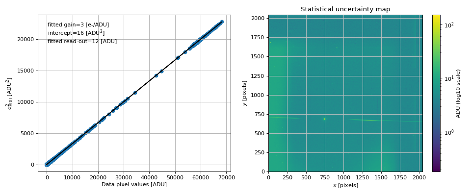
check_statistical_error()[source]

Check that statistical uncertainty map follows the input uncertainty model in terms of gain and read-out noise.

A linear model is fitted to the squared pixel uncertainty values with respect to the pixel data values. The slop gives the gain value and the intercept gives the read-out noise value.

Returns:

fit (tuple) – The best fit parameter of the linear model.
x (array_like) – The x data used for the fit (data).
y (array_like) – The y data used for the fit (squared uncertainties).
model (array_like) – The linear model values.

Examples

>>> im = Image('tests/data/reduc_20170530_134.fits')
>>> im.convert_to_ADU_units()
>>> fit, x, y, model = im.check_statistical_error()

compute_parallactic_angle()[source]

Compute the parallactic angle.

Script from A. Guyonnet.

compute_statistical_error()[source]

Compute the image noise map from Image.data. The latter must be in ADU. The function first converts the image in electron counts units, evaluate the Poisson noise, add in quadrature the read-out noise, takes the square root and returns a map in ADU units.

Examples

>>> im = Image('tests/data/reduc_20170530_134.fits', config="./config/ctio.ini")
>>> im.convert_to_ADU_units()
>>> im.compute_statistical_error()
>>> im.plot_statistical_error()

(Source code)

convert_to_ADU_rate_units()[source]

Convert Image data from ADU to ADU/s units.

Examples

>>> im = Image('tests/data/reduc_20170605_028.fits')
>>> print(im.expo)
600.0
>>> data_before = np.copy(im.data)
>>> im.convert_to_ADU_rate_units()

convert_to_ADU_units()[source]

Convert Image data from ADU/s to ADU units.

Examples

>>> im = Image('tests/data/reduc_20170605_028.fits')
>>> print(im.expo)
600.0
>>> data_before = np.copy(im.data)
>>> im.convert_to_ADU_rate_units()
>>> data_after = np.copy(im.data)
>>> im.convert_to_ADU_units()

load_image(file_name)[source]

Load the image and store some information from header in class attributes. Then load the target and disperser properties. Called when an Image instance is created.

Parameters:: file_name (str) – The fits file name.

plot_image(ax=None, scale='lin', title='', units='', plot_stats=False, target_pixcoords=None, figsize=(7.3, 6), aspect=None, vmin=None, vmax=None, cmap=None, cax=None, use_flat=True)[source]

Plot image.

Parameters:

ax (Axes, optional) – Axes instance (default: None).
scale (str) – Scaling of the image (choose between: lin, log or log10, symlog) (default: lin)
title (str) – Title of the image (default: “”)
units (str) – Units of the image to be written in the color bar label (default: “”)
cmap (colormap) – Color map label (default: None)
target_pixcoords (array_like, optional) – 2D array giving the (x,y) coordinates of the targets on the image: add a scatter plot (default: None)
vmin (float) – Minimum value of the image (default: None)
vmax (float) – Maximum value of the image (default: None)
aspect (str) – Aspect keyword to be passed to imshow (default: None)
cax (Axes, optional) – Color bar axes if necessary (default: None).
figsize (tuple) – Figure size (default: [9.3, 8]).
plot_stats (bool) – If True, plot the uncertainty map instead of the image (default: False).
use_flat (bool) – If True and self.flat exists, divide the image by the flat (default: True).

Examples

>>> im = Image('tests/data/reduc_20170605_028.fits', config="./config/ctio.ini")
>>> im.mask = np.zeros_like(im.data).astype(bool)
>>> im.mask[700:705, 1250:1260] = True  # test masking of some pixels like cosmic rays
>>> im.plot_image(target_pixcoords=[820, 580], scale="symlog")
>>> if parameters.DISPLAY: plt.show()

plot_statistical_error()[source]

Plot the statistical uncertainty map and check it is a Poisson noise.

The image units must be ADU.

Examples

>>> im = Image('tests/data/reduc_20170530_134.fits')
>>> im.convert_to_ADU_units()
>>> im.plot_statistical_error()

(Source code)

rebin()[source]

Rebin the image and reset some related parameters.

Examples

>>> parameters.CCD_REBIN = 2
>>> im = Image('tests/data/reduc_20170605_028.fits')
>>> im.mask = np.zeros_like(im.data).astype(bool)
>>> im.mask[700:750, 800:850] = True
>>> im.target_guess = [810, 590]
>>> im.data.shape
(2048, 2048)
>>> im.rebin()
>>> im.data.shape
(1024, 1024)
>>> im.err.shape
(1024, 1024)
>>> im.target_guess
array([405., 295.])

save_image(output_file_name, overwrite=False)[source]

Save the image in a fits file.

Parameters:

output_file_name (str) – The output file name.
overwrite (bool) – If True, overwrite the file if it exists previously (default: False).

Examples

>>> im = Image('tests/data/reduc_20170605_028.fits')
>>> im.save_image('tests/data/reduc_20170605_028_copy.fits', overwrite=True)

simulate_starfield_with_gaia()[source]

spectractor.extractor.images.build_CTIO_gain_map(image)[source]

Compute the CTIO gain map according to header GAIN values.

Parameters:: image (Image) – The Image instance to fill with file data and header.

spectractor.extractor.images.build_CTIO_read_out_noise_map(image)[source]

Compute the CTIO gain map according to header GAIN values.

Parameters:: image (Image) – The Image instance to fill with file data and header.

spectractor.extractor.images.compute_rotation_angle_hessian(image, angle_range=(-10, 10), width_cut=100, edges=(0, 2048), margin_cut=12, pixel_fraction=0.01)[source]

Compute the rotation angle in degree of a spectrogram with the Hessian of the image. Use the disperser rotation angle map as a prior and the target_pixcoords values to crop the image around the spectrogram.

Parameters:

image (Image) – The Image instance.
angle_range ((float, float)) – Don’t consider pixel with Hessian angle outside this range (default: (-10,10)).
width_cut (int) – Half with of the image to consider in height (default: parameters.YWINDOW).
edges ((int, int)) – Minimum and maximum pixel on the right edge (default: (0, parameters.CCD_IMSIZE)).
margin_cut (int) – After computing the Hessian, to avoid bad values on the edges the function cut on the edge of image margin_cut pixels (default: 12).
pixel_fraction (float) – Minimum pixel fraction to keep after thresholding the lambda minus map (default: 0.01).

Returns:

theta – The median value of the histogram of angles deduced with the Hessian of the pixels (in degree).

Return type:

float

Examples

>>> im=Image('tests/data/reduc_20170605_028.fits', disperser_label='HoloPhAg')

Create a mock spectrogram:

>>> from scipy.ndimage import gaussian_filter
>>> N = parameters.CCD_IMSIZE
>>> im.data = np.ones((N, N))
>>> slope = -0.1
>>> y = lambda x: slope * (x - 0.5*N) + 0.5*N
>>> for x in np.arange(N):
...     im.data[int(y(x)), x] = 100
...     im.data[int(y(x))+1, x] = 100
>>> im.data = gaussian_filter(im.data, sigma=5)
>>> im.target_pixcoords=(N//2, N//2)
>>> parameters.DEBUG = True
>>> theta = compute_rotation_angle_hessian(im)

spectractor.extractor.images.find_target(image, guess=None, rotated=False, widths=[100, 100])[source]

Find the target in the Image instance.

The object is search in a windows of size defined by the XWINDOW and YWINDOW parameters, using two iterative fits of a PSF model. User must give a guess array in the raw image.

Parameters:

image (Image) – The Image instance.
guess (array_like) – Two parameter array giving the estimated position of the target in the image, optional if WCS is used.
rotated (bool) – If True, the target is searched in the rotated image.
widths ((int, int)) – Two parameter array to define the width of the cropped image (default: [parameters.XWINDOW, parameters.YWINDOW])

Returns:

x0 (float) – The x position of the target.
y0 (float) – The y position of the target.

Examples

>>> parameters.CCD_REBIN = 1
>>> im = Image('tests/data/reduc_20170530_134.fits', target_label="HD111980", config="./config/ctio.ini")
>>> im.plot_image(scale="symlog")
>>> guess = [750, 680]
>>> parameters.VERBOSE = True
>>> parameters.DEBUG = True
>>> parameters.SPECTRACTOR_FIT_TARGET_CENTROID = "fit"
>>> find_target(im, guess)  
[743.7... 683.1...]
>>> parameters.SPECTRACTOR_FIT_TARGET_CENTROID = "WCS"
>>> find_target(im, guess)  
[745... 684...]
>>> parameters.SPECTRACTOR_FIT_TARGET_CENTROID = "guess"
>>> find_target(im, guess, widths=(100, 100))
[750, 680]

spectractor.extractor.images.find_target_1Dprofile(image, sub_image, guess)[source]

Find precisely the position of the targeted object fitting a PSF model on each projection of the image along x and y, using outlier removal.

Parameters:

image (Image) – The Image instance.
sub_image (array_like) – The cropped image data array where the fit is performed.
guess (array_like) – Two parameter array giving the estimated position of the target in the image.

Examples

>>> im = Image('tests/data/reduc_20170605_028.fits')
>>> guess = [820, 580]
>>> parameters.DEBUG = True
>>> sub_image, x0, y0, Dx, Dy, sub_errors = find_target_init(im, guess, rotated=False)
>>> x1, y1 = find_target_1Dprofile(im, sub_image, guess)

spectractor.extractor.images.find_target_Moffat2D(image, sub_image_subtracted, sub_errors=None)[source]

Find precisely the position of the targeted object fitting a Moffat PSF model. A polynomial 2D background is subtracted first. Saturated pixels are masked with np.nan values.

Parameters:

image (Image) – The Image instance.
sub_image_subtracted (array_like) – The cropped image data array where the fit is performed, background has been subtracted.
sub_errors (array_like) – The image data uncertainties.

Examples

>>> im = Image('tests/data/reduc_20170605_028.fits')
>>> guess = [820, 580]
>>> parameters.VERBOSE = True
>>> parameters.DEBUG = True
>>> sub_image_subtracted, x0, y0, Dx, Dy, sub_errors = find_target_init(im, guess, rotated=False) #, widths=[30,30])
>>> xmax = np.argmax(np.sum(sub_image_subtracted, axis=0))
>>> ymax = np.argmax(np.sum(sub_image_subtracted, axis=1))
>>> x1, y1 = find_target_Moffat2D(im, sub_image_subtracted, sub_errors=sub_errors)

spectractor.extractor.images.find_target_after_rotation(image)[source]

spectractor.extractor.images.find_target_init(image, guess, rotated=False, widths=[100, 100])[source]

Initialize the search of the target: crop the image, set the saturation level, estimate and subtract a 2D polynomial background.

Parameters:

image (Image) – The Image instance.
guess (array_like) – Two parameter array giving the estimated position of the target in the image.
rotated (bool) – If True, the target is searched in the rotated image.
widths ((int, int)) – Two parameter array to define the width of the cropped image (default: [parameters.XWINDOW, parameters.YWINDOW])

Returns:

sub_image (array_like) – The cropped image data array where the fit has to be performed.
x0 (float) – The x position of the target.
y0 (float) – The y position of the target.
Dx (int) – The width of the cropped image.
Dy (int) – The height of the cropped image.
sub_errors (array_like) – The cropped image uncertainty array where the fit has to be performed.

spectractor.extractor.images.load_AUXTEL_image(image)[source]

Specific routine to load AUXTEL fits files and load their data and properties for Spectractor.

Parameters:: image (Image) – The Image instance to fill with file data and header.

spectractor.extractor.images.load_CTIO_image(image)[source]

Specific routine to load CTIO fits files and load their data and properties for Spectractor.

Parameters:: image (Image) – The Image instance to fill with file data and header.

spectractor.extractor.images.load_LPNHE_image(image)[source]

Specific routine to load LPNHE fits files and load their data and properties for Spectractor.

Parameters:: image (Image) – The Image instance to fill with file data and header.

spectractor.extractor.images.load_STARDICE_image(image)[source]

Specific routine to load STARDICE fits files and load their data and properties for Spectractor.

Parameters:: image (Image) – The Image instance to fill with file data and header.

spectractor.extractor.images.turn_image(image)[source]

Compute the rotation angle using the Hessian algorithm and turn the image.

The results are stored in Image.data_rotated and Image.stat_errors_rotated.

Parameters:: image (Image) – The Image instance.
Returns:: rotation_angle – Rotation angle in degree.
Return type:: float

Examples

Create of False spectrogram:

>>> im=Image('tests/data/reduc_20170605_028.fits', disperser_label='HoloPhAg')
>>> N = parameters.CCD_IMSIZE
>>> im.data = np.ones((N, N))
>>> slope = -0.1
>>> y = lambda x: slope * (x - 0.5*N) + 0.5*N
>>> for x in np.arange(N):
...     im.data[int(y(x)), x] = 10
...     im.data[int(y(x))+1, x] = 10

(Source code)

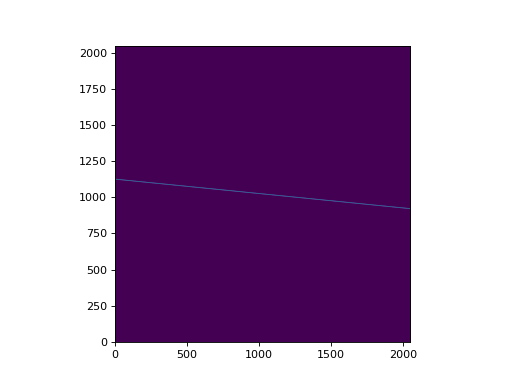
>>> im.target_pixcoords=(N//2, N//2)
>>> parameters.DEBUG = True
>>> parameters.SPECTRACTOR_COMPUTE_ROTATION_ANGLE = False
>>> turn_image(im)
0
>>> parameters.SPECTRACTOR_COMPUTE_ROTATION_ANGLE = "disperser"
>>> turn_image(im)
-1.915
>>> parameters.SPECTRACTOR_COMPUTE_ROTATION_ANGLE = "hessian"
>>> turn_image(im)  
-5.90...

(Source code)

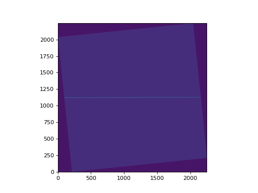
spectractor.extractor.psf module

class spectractor.extractor.psf.DoubleMoffat(values=None, clip=False)[source]

Bases: PSF

apply_max_width_to_bounds(max_half_width=None)[source]

evaluate(pixels, values=None)[source]

Evaluate the DoubleMoffat function.

The function is normalized to have an integral equal to amplitude parameter, with normalisation factor:

\[f(y) \propto \frac{A}{ \frac{\Gamma(\alpha_1)}{\gamma_1 \sqrt{\pi} \Gamma(\alpha_1 -1/2)}+\eta\frac{\Gamma(\alpha_2)}{\gamma_2 \sqrt{\pi} \Gamma(\alpha_2 -1/2)}, \quad \int_{y_{\text{min}}}^{y_{\text{max}}} f(y) \mathrm{d}y = A\]

Parameters:

pixels (list) – List containing the X abscisse 2D array and the Y abscisse 2D array.
values (array_like) – The parameter array. If None, the array used to instanciate the class is taken. If given, the class instance parameter array is updated.

Returns:

output – The PSF function evaluated.

Return type:

array_like

Examples

>>> p = [2,20,30,4,2,2,5,1.5,20]
>>> psf = DoubleMoffat(p)
>>> yy, xx = np.mgrid[:50, :60]
>>> out = psf.evaluate(pixels=np.array([xx, yy]), values=p)

(Source code)

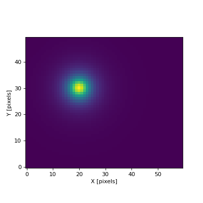
jacobian(pixels, params, epsilon=None, model_input=None, analytical=True)[source]

Evaluate the PSF DoubleMoffat Jacobian.

The function is normalized to have an integral equal to amplitude parameter, with normalisation factor:

Parameters:

pixels (array_like) – List containing the X abscisse 2D array and the Y abscisse 2D array.
params (array_like) – The parameter array. If None, the array used to instanciate the class is taken. If given, the class instance parameter array is updated.
epsilon (array_like, optional) – The array of small steps to compute the partial derivatives of the model if analytical=False (default: None).
model_input (array_like, optional) – A model input as a list with (x, model, model_err) to avoid an additional call to simulate() if analytical=False (default: None).
analytical (bool, optional) – If True, use analytical derivatives to compute Jacobian operator. Otherwise use numerical differenciations with steps given by epsilon argument (default: True).

Returns:

jacobian – The PSF Jacobian.

Return type:

array_like

Examples

>>> p = [2,20,30,4,2,0.5,3,3,20]
>>> epsilon = [0.001] * len(p)
>>> psf = DoubleMoffat(p)
>>> psf.params.fixed = [True, True, False, False, False, False, False, False, True]  # fix amplitude, x_c, saturation

2D case

>>> yy, xx = np.mgrid[:50, :60]
>>> J_ana = psf.jacobian(pixels=np.array([xx, yy]), params=p, epsilon=epsilon, analytical=True)
>>> J_num = psf.jacobian(pixels=np.array([xx, yy]), params=p, epsilon=epsilon, analytical=False)
>>> np.allclose(J_num, J_ana, rtol=1e-4, atol=1e-4)
True
>>> np.allclose(J_ana[0:2], 0)
True

1D case

>>> y = np.mgrid[:50]
>>> J_ana = psf.jacobian(pixels=y, params=p, epsilon=epsilon, analytical=True)
>>> J_num = psf.jacobian(pixels=y, params=p, epsilon=epsilon, analytical=False)
>>> np.allclose(J_num, J_ana, rtol=1e-3, atol=1e-3)
True
>>> np.allclose(J_ana[0:2], 0)
True

class spectractor.extractor.psf.Gauss(values=None, clip=False)[source]

Bases: PSF

apply_max_width_to_bounds(max_half_width=None)[source]

evaluate(pixels, values=None)[source]

Evaluate the Gauss function.

The function is normalized to have an integral equal to amplitude parameter, with normalisation factor:

Parameters:

pixels (list) – List containing the X abscisse 2D array and the Y abscisse 2D array.
values (array_like) – The parameter array. If None, the array used to instanciate the class is taken. If given, the class instance parameter array is updated.

Returns:

output – The PSF function evaluated.

Return type:

array_like

Examples

>>> p = [2,20,30,2,10]
>>> psf = Gauss(p, clip=True)
>>> yy, xx = np.mgrid[:50, :60]
>>> out = psf.evaluate(pixels=np.array([xx, yy]), values=p)

(Source code)

jacobian(pixels, params, epsilon=None, model_input=None, analytical=True)[source]

Evaluate the PSF Gauss Jacobian.

The function is normalized to have an integral equal to amplitude parameter, with normalisation factor:

Parameters:

pixels (array_like) – List containing the X abscisse 2D array and the Y abscisse 2D array.
params (array_like) – The parameter array. If None, the array used to instanciate the class is taken. If given, the class instance parameter array is updated.
epsilon (array_like, optional) – The array of small steps to compute the partial derivatives of the model if analytical=False (default: None).
model_input (array_like, optional) – A model input as a list with (x, model, model_err) to avoid an additional call to simulate() if analytical=False (default: None).
analytical (bool, optional) – If True, use analytical derivatives to compute Jacobian operator. Otherwise use numerical differenciations with steps given by epsilon argument (default: True).

Returns:

jacobian – The PSF Jacobian.

Return type:

array_like

Examples

>>> p = [2,20,30,2,10]
>>> epsilon = [0.001] * len(p)
>>> psf = Gauss(p, clip=True)
>>> psf.params.fixed = [True, True, False, False, True]  # fix amplitude, x_c, saturation

2D case

>>> yy, xx = np.mgrid[:50, :60]
>>> J_ana = psf.jacobian(pixels=np.array([xx, yy]), params=p, epsilon=epsilon, analytical=True)
>>> J_num = psf.jacobian(pixels=np.array([xx, yy]), params=p, epsilon=epsilon, analytical=False)
>>> np.allclose(J_num, J_ana, rtol=1e-2, atol=1e-4)
True
>>> np.allclose(J_ana[0:2], 0)
True

1D case

>>> y = np.mgrid[:50]
>>> J_ana = psf.jacobian(pixels=y, params=p, epsilon=epsilon, analytical=True)
>>> J_num = psf.jacobian(pixels=y, params=p, epsilon=epsilon, analytical=False)
>>> np.allclose(J_num, J_ana, rtol=1e-2, atol=1e-4)
True
>>> np.allclose(J_ana[0:2], 0)
True

class spectractor.extractor.psf.Moffat(values=None, clip=False)[source]

Bases: PSF

apply_max_width_to_bounds(max_half_width=None)[source]

evaluate(pixels, values=None)[source]

Evaluate the Moffat function.

The function is normalized to have an integral equal to amplitude parameter, with normalisation factor:

\[f(y) \propto \frac{A \Gamma(\alpha)}{\gamma \sqrt{\pi} \Gamma(\alpha -1/2)}, \quad \int_{y_{\text{min}}}^{y_{\text{max}}} f(y) \mathrm{d}y = A\]

Parameters:

pixels (list) – List containing the X abscisse 2D array and the Y abscisse 2D array.
values (array_like) – The parameter array. If None, the array used to instanciate the class is taken. If given, the class instance parameter array is updated.

Returns:

output – The PSF function evaluated.

Return type:

array_like

Examples

>>> p = [2,20,30,4,2,10]
>>> psf = Moffat(p, clip=True)
>>> yy, xx = np.mgrid[:50, :60]
>>> output = psf.evaluate(pixels=np.array([xx, yy]), values=p)

>>> p = [2,20,30,4,2,10]
>>> psf = Moffat(p, clip=True)
>>> xx = np.arange(0, 50, 1)
>>> output = psf.evaluate(pixels=xx, values=p)

(Source code)

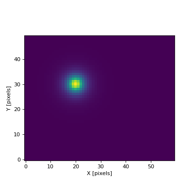
jacobian(pixels, params, epsilon=None, model_input=None, analytical=True)[source]

Evaluate the PSF Moffat Jacobian.

The function is normalized to have an integral equal to amplitude parameter, with normalisation factor:

Parameters:

pixels (array_like) – List containing the X abscisse 2D array and the Y abscisse 2D array.
params (array_like) – The parameter array. If None, the array used to instanciate the class is taken. If given, the class instance parameter array is updated.
epsilon (array_like, optional) – The array of small steps to compute the partial derivatives of the model if analytical=False (default: None).
model_input (array_like, optional) – A model input as a list with (x, model, model_err) to avoid an additional call to simulate() if analytical=False (default: None).
analytical (bool, optional) – If True, use analytical derivatives to compute Jacobian operator. Otherwise use numerical differenciations with steps given by epsilon argument (default: True).

Returns:

jacobian – The PSF Jacobian.

Return type:

array_like

Examples

>>> p = [2,20,30,4,2,10]
>>> epsilon = [0.01] * len(p)
>>> psf = Moffat(p, clip=True)
>>> psf.params.fixed = [True, True, False, False, False, True]  # fix amplitude, x_c, saturation

2D case

>>> yy, xx = np.mgrid[:50, :60]
>>> J_ana = psf.jacobian(pixels=np.array([xx, yy]), params=p, epsilon=epsilon, analytical=True)
>>> J_num = psf.jacobian(pixels=np.array([xx, yy]), params=p, epsilon=epsilon, analytical=False)
>>> np.allclose(J_num, J_ana, rtol=1e-4, atol=1e-4)
True
>>> np.allclose(J_ana[0:2], 0)
True

1D case

>>> y = np.mgrid[:50]
>>> J_ana = psf.jacobian(pixels=y, params=p, epsilon=epsilon, analytical=True)
>>> J_num = psf.jacobian(pixels=y, params=p, epsilon=epsilon, analytical=False)
>>> np.allclose(J_num, J_ana, rtol=1e-3, atol=1e-3)
True
>>> np.allclose(J_ana[0:2], 0)
True

class spectractor.extractor.psf.MoffatGauss(values=None, clip=False)[source]

Bases: PSF

apply_max_width_to_bounds(max_half_width=None)[source]

evaluate(pixels, values=None)[source]

Evaluate the MoffatGauss function.

The function is normalized to have an integral equal to amplitude parameter, with normalisation factor:

\[f(y) \propto \frac{A}{ \frac{\Gamma(\alpha)}{\gamma \sqrt{\pi} \Gamma(\alpha -1/2)}+\eta\sqrt{2\pi}\sigma}, \quad \int_{y_{\text{min}}}^{y_{\text{max}}} f(y) \mathrm{d}y = A\]

Parameters:

pixels (list) – List containing the X abscisse 2D array and the Y abscisse 2D array.
values (array_like) – The parameter array. If None, the array used to instanciate the class is taken. If given, the class instance parameter array is updated.

Returns:

output – The PSF function evaluated.

Return type:

array_like

Examples

>>> p = [2,20,30,4,2,-0.5,1,10]
>>> psf = MoffatGauss(p)
>>> yy, xx = np.mgrid[:50, :60]
>>> out = psf.evaluate(pixels=np.array([xx, yy]), values=p)

(Source code)

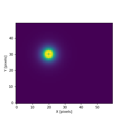
jacobian(pixels, params, epsilon=None, model_input=None, analytical=True)[source]

Evaluate the PSF Moffat+Gauss Jacobian.

The function is normalized to have an integral equal to amplitude parameter, with normalisation factor:

Parameters:

pixels (array_like) – List containing the X abscisse 2D array and the Y abscisse 2D array.
params (array_like) – The parameter array. If None, the array used to instanciate the class is taken. If given, the class instance parameter array is updated.
epsilon (array_like, optional) – The array of small steps to compute the partial derivatives of the model if analytical=False (default: None).
model_input (array_like, optional) – A model input as a list with (x, model, model_err) to avoid an additional call to simulate() if analytical=False (default: None).
analytical (bool, optional) – If True, use analytical derivatives to compute Jacobian operator. Otherwise use numerical differenciations with steps given by epsilon argument (default: True).

Returns:

jacobian – The PSF Jacobian.

Return type:

array_like

Examples

>>> p = [2,20,30,4,2,-0.5,1,10]
>>> epsilon = [0.001] * len(p)
>>> psf = MoffatGauss(p)
>>> psf.params.fixed = [True, True, False, False, False, False, False, True]  # fix amplitude, x_c, saturation

2D case

>>> yy, xx = np.mgrid[:50, :60]
>>> J_ana = psf.jacobian(pixels=np.array([xx, yy]), params=p, epsilon=epsilon, analytical=True)
>>> J_num = psf.jacobian(pixels=np.array([xx, yy]), params=p, epsilon=epsilon, analytical=False)
>>> np.allclose(J_num, J_ana, rtol=1e-4, atol=1e-4)
True
>>> np.allclose(J_ana[0:2], 0)
True

1D case

>>> y = np.mgrid[:50]
>>> J_ana = psf.jacobian(pixels=y, params=p, epsilon=epsilon, analytical=True)
>>> J_num = psf.jacobian(pixels=y, params=p, epsilon=epsilon, analytical=False)
>>> np.allclose(J_num, J_ana, rtol=1e-3, atol=1e-3)
True
>>> np.allclose(J_ana[0:2], 0)
True

class spectractor.extractor.psf.Order0(target, values=None, clip=False)[source]

Bases: PSF

apply_max_width_to_bounds(max_half_width=None)[source]

build_interpolated_functions(target)[source]

Interpolate the order 0 image and make 1D and 2D functions centered on its centroid, with varying width and normalized to get an integral equal to unity.

Parameters:: target (Target) – The target with a target.image attribute to interpolate.
Returns:: func – The 2D interpolated function centered in (target.image_x0, target.image_y0).
Return type:: Callable

evaluate(pixels, values=None)[source]

Evaluate the Order 0 interpolated function.

The function is normalized to have an integral equal to amplitude parameter.

Parameters:

pixels (list) – List containing the X abscisse 2D array and the Y abscisse 2D array.
values (array_like) – The parameter array. If None, the array used to instanciate the class is taken. If given, the class instance parameter array is updated.

Returns:

output – The PSF function evaluated.

Return type:

array_like

Examples

>>> from spectractor.extractor.images import Image, find_target
>>> im = Image('tests/data/reduc_20170605_028.fits', target_label="PNG321.0+3.9")
>>> im.plot_image()
>>> guess = [820, 580]
>>> parameters.VERBOSE = True
>>> parameters.DEBUG = True
>>> x0, y0 = find_target(im, guess)

>>> p = [1,40,50,1,1e20]
>>> psf = Order0(target=im.target)

2D evaluation:

>>> yy, xx = np.mgrid[:80, :100]
>>> out = psf.evaluate(pixels=np.array([xx, yy]), values=p)

1D evaluation:

>>> out = psf.evaluate(pixels=np.arange(100), values=p)

(Source code)

jacobian(pixels, params, epsilon=None, model_input=None, analytical=False)[source]

Evaluate the PSF Order0 Jacobian. Analytical Jacobian is not available.

The function is normalized to have an integral equal to amplitude parameter, with normalisation factor:

Parameters:

pixels (array_like) – List containing the X abscisse 2D array and the Y abscisse 2D array.
params (array_like) – The parameter array. If None, the array used to instanciate the class is taken. If given, the class instance parameter array is updated.
epsilon (array_like, optional) – The array of small steps to compute the partial derivatives of the model if analytical=False (default: None).
model_input (array_like, optional) – A model input as a list with (x, model, model_err) to avoid an additional call to simulate() if analytical=False (default: None).
analytical (bool, optional) – If True, use analytical derivatives to compute Jacobian operator. Otherwise use numerical differenciations with steps given by epsilon argument (default: True).

Returns:

jacobian – The PSF Jacobian.

Return type:

array_like

Examples

>>> from spectractor.extractor.images import Image, find_target
>>> im = Image('tests/data/reduc_20170530_134.fits', target_label="HD111980")
>>> im.plot_image()
>>> guess = [820, 580]
>>> parameters.VERBOSE = True
>>> parameters.DEBUG = True
>>> x0, y0 = find_target(im, guess)

>>> p = [1,40,50,1,1e20]
>>> psf = Order0(target=im.target, values=p)

>>> epsilon = [0.01] * len(p)
>>> psf.params.fixed[2] = True  # fix y_c
>>> psf.params.fixed = [True, True, False, False, True]  # fix amplitude, x_c, saturation
>>> yy, xx = np.mgrid[:50, :60]
>>> J_num = psf.jacobian(pixels=np.array([xx, yy]), params=p, epsilon=epsilon, analytical=False)
>>> J_num.shape
(5, 3000)
>>> np.sum(J_num[2])
0.0
>>> np.allclose(J_num[0:2], 0)
True

class spectractor.extractor.psf.PSF(clip=False)[source]

Bases: object

Generic PSF model class.

The PSF models must contain at least the “amplitude”, “x_c” and “y_c” parameters as the first three parameters (in this order) and “saturation” parameter as the last parameter. “amplitude”, “x_c” and “y_c” stands respectively for the general amplitude of the model, the position along the dispersion axis and the transverse position with respect to the dispersion axis (assumed to be the X axis). Last “saturation” parameter must be express in the same units as the signal to model and as the “amplitude” parameter. The PSF models must be normalized to one in total flux divided by the first parameter (amplitude). Then the PSF model integral is equal to the “amplitude” parameter.

apply_max_width_to_bounds(max_half_width=None)[source]

evaluate(pixels, values=None)[source]

fit_psf(data, data_errors=None, bgd_model_func=None)[source]

Fit a PSF model on 1D or 2D data.

Parameters:

data (array_like) – 1D or 2D array containing the data.
data_errors (np.array, optional) – The 1D or 2D array of uncertainties.
bgd_model_func (callable, optional) – A 1D or 2D function to model the extracted background (default: None -> null background).

Returns:

fit_workspace – The PSFFitWorkspace instance to get info about the fitting.

Return type:

PSFFitWorkspace

Examples

Build a mock PSF2D without background and with random Poisson noise:

>>> p0 = np.array([200000, 20, 30, 5, 2, -0.1, 2, 400000])
>>> psf0 = MoffatGauss(p0)
>>> yy, xx = np.mgrid[:50, :60]
>>> data = psf0.evaluate(np.array([xx, yy]), p0)
>>> data = np.random.poisson(data)
>>> data_errors = np.sqrt(data+1)

Fit the data in 2D:

>>> p = np.array([150000, 19, 31, 4.5, 2.5, -0.1, 3, 400000])
>>> psf = MoffatGauss(p)
>>> w = psf.fit_psf(data, data_errors=data_errors, bgd_model_func=None)
>>> w.plot_fit()

Fit the data in 1D:

>>> data1d = data[:,int(p0[1])]
>>> data1d_err = data_errors[:,int(p0[1])]
>>> p = np.array([10000, 20, 32, 4, 3, -0.1, 2, 400000])
>>> psf1d = MoffatGauss(p)
>>> w = psf1d.fit_psf(data1d, data_errors=data1d_err, bgd_model_func=None)
>>> w.plot_fit()

(Source code)

jacobian(pixels, params, epsilon=None, model_input=None, analytical=True)[source]

class spectractor.extractor.psf.PSFFitWorkspace(psf, data, data_errors, bgd_model_func=None, jacobian_analytical=False, file_name='', verbose=False, plot=False, live_fit=False, truth=None)[source]

Bases: FitWorkspace

Generic PSF fitting workspace.

jacobian(params, model_input=None)[source]

Compute the Jacobian matrix of a PSF model, with analytical derivatives if they exist, numerical derivatives otherwise.

Parameters:

params (array_like) – The array of model parameters.
model_input (array_like, optional) – A model input as a list with (x, model, model_err) to avoid an additional call to simulate().

Returns:

J – The Jacobian matrix.

Return type:

np.array

plot_fit()[source]

Generic function to plot the result of the fit for 1D curves.

Returns:: fig – The figure.
Return type:: plt.FigureClass

simulate(*psf_params)[source]

Compute a PSF model given PSF parameters and minimizing amplitude parameter given a data array.

Parameters:: psf_params (array_like) – PSF shape parameter array (all parameters except amplitude).

Examples

Build a mock PSF2D without background and with random Poisson noise:

>>> p = np.array([200000, 20, 30, 5, 2, -0.1, 2, 400000])
>>> psf = MoffatGauss(p)
>>> yy, xx = np.mgrid[:50, :60]
>>> data = psf.evaluate(np.array([xx, yy]), p)
>>> data = np.random.poisson(data)
>>> data_errors = np.sqrt(data+1)

Fit the data in 2D:

>>> w = PSFFitWorkspace(psf, data, data_errors, bgd_model_func=None, verbose=True)
>>> x, mod, mod_err = w.simulate(*p)
>>> w.plot_fit()

Fit the data in 1D:

>>> data1d = data[:,int(p[1])]
>>> data1d_err = data_errors[:,int(p[1])]
>>> psf.params.values[0] = p[0] / 10.5
>>> w = PSFFitWorkspace(psf, data1d, data1d_err, bgd_model_func=None, verbose=True)
>>> x, mod, mod_err = w.simulate(*psf.params.values)
>>> w.plot_fit()

(Source code)

spectractor.extractor.psf.evaluate_doublemoffat1d(y, amplitude, y_c, gamma1, alpha1, eta, gamma2, alpha2, norm1, norm2)[source]

Compute a 1D DoubleMoffat function, whose integral is normalised to unity.

\[f(y) \propto A \left\lbrace \frac{1}{\left[ 1 +\left(\frac{y-y_c}{\gamma}\right)^2 \right]^\alpha}+ \eta e^{-(y-y_c)^2/(2\sigma^2)}\right\rbrace \quad\text{ and } \quad \eta < 0, \alpha > 1/2\]

Note that this function is defined only for \(\alpha > 1/2\). The normalisation factor for the Moffat+Gauss \(\frac{\Gamma(\alpha)}{\gamma \sqrt{\pi} \Gamma(\alpha -1/2)} + \eta \sqrt{2\pi} \sigma\) is not included as special functions are not supproted by the numba library.

Parameters:

y (array_like) – 1D array of pixels \(y\), regularly spaced.
amplitude (float) – Integral \(A\) of the function.
y_c (float) – Center \(y_c\) of the function.
gamma1 (float) – Width \(\gamma_1\) of the Moffat function.
alpha1 (float) – Exponent \(\alpha_1\) of the Moffat function.
eta (float) – Relative amplitude of the second Moffat function.
gamma2 (float) – Width \(\gamma_2\) of the second Moffat function.
alpha2 (float) – Exponent \(\alpha_2\) of the second Moffat function.
norm1 (float) – Normalisation \(\frac{\Gamma(\alpha_1)}{\gamma_1 \sqrt{\pi} \Gamma(\alpha_1 -1/2)}\).
norm2 (float) – Normalisation \(\frac{\Gamma(\alpha_2)}{\gamma_2 \sqrt{\pi} \Gamma(\alpha_2 -1/2)}\).

Returns:

output – 1D array of the function evaluated on the y pixel array.

Return type:

array_like

Examples

>>> Ny = 50
>>> y = np.arange(Ny)
>>> amplitude = 10
>>> gamma1 = 5
>>> alpha1 = 2
>>> eta = 2
>>> gamma2 = 4
>>> alpha2 = 3
>>> norm1 = evaluate_moffat1d_normalisation(gamma1, alpha1)
>>> norm2 = evaluate_moffat1d_normalisation(gamma2, alpha2)
>>> a = evaluate_doublemoffat1d(y, amplitude=amplitude, y_c=Ny/2, gamma1=gamma1, alpha1=alpha1, eta=eta, gamma2=gamma2, alpha2=alpha2, norm1=norm1, norm2=norm2)
>>> print(f"{np.sum(a):.6f}")
9.985071
>>> a.dtype
dtype('float32')

(Source code)

spectractor.extractor.psf.evaluate_doublemoffat1d_jacobian(y, amplitude, y_c, gamma1, alpha1, eta, gamma2, alpha2, norm1, dnormda1, norm2, dnormda2, fixed)[source]

Compute a 1D DoubleMoffat Jacobian, whose integral is normalised to unity.

\[f(y) \propto A \left\lbrace \frac{1}{\left[ 1 +\left(\frac{y-y_c}{\gamma}\right)^2 \right]^\alpha} \times \frac{\Gamma(\alpha)}{\gamma \sqrt{\pi} \Gamma(\alpha -1/2)} - \eta e^{-(y-y_c)^2/(2\sigma^2)}\right\rbrace \quad\text{ and } \quad \eta < 0, \alpha > 1/2\]

Note that this function is defined only for \(\alpha > 1/2\). The normalisation factor for the Moffat \(\frac{\Gamma(\alpha)}{\gamma \sqrt{\pi} \Gamma(\alpha -1/2)} + \eta \sqrt{2\pi} \sigma\) is not included as special functions are not supproted by the numba library.

Parameters:

y (array_like) – 1D array of pixels \(y\), regularly spaced.
amplitude (float) – Integral \(A\) of the function.
y_c (float) – Center \(y_c\) of the function.
gamma1 (float) – Width \(\gamma_1\) of the Moffat function.
alpha1 (float) – Exponent \(\alpha_1\) of the Moffat function.
eta (float) – Relative amplitude of the second Moffat function.
gamma2 (float) – Width \(\gamma_2\) of the second Moffat function.
alpha2 (float) – Exponent \(\alpha_2\) of the second Moffat function.
norm1 (float) – Normalisation \(\frac{\Gamma(\alpha_1)}{\gamma_1 \sqrt{\pi} \Gamma(\alpha_1 -1/2)}\).
dnormda1 (float) – Derivatives of the normalisation with respect to alpha1.
norm2 (float) – Normalisation \(\frac{\Gamma(\alpha_2)}{\gamma_2 \sqrt{\pi} \Gamma(\alpha_2 -1/2)}\).
dnormda2 (float) – Derivatives of the normalisation with respect to alpha2.
fixed (array_like) – Array of booleans, with True values for fixed parameters.

Returns:

J – 2D array of the model Jacobian.

Return type:

array_like

Examples

>>> Ny = 50
>>> y = np.arange(Ny)
>>> amplitude = 10
>>> gamma1 = 5
>>> alpha1 = 2
>>> gamma2 = 4
>>> alpha2 = 3
>>> eta = 2
>>> norm1 = evaluate_moffat1d_normalisation(gamma1, alpha1)
>>> dnormda1 = evaluate_moffat1d_normalisation_dalpha(norm1, alpha1)
>>> norm2 = eta * evaluate_moffat1d_normalisation(gamma2, alpha2)
>>> dnormda2 = evaluate_moffat1d_normalisation_dalpha(norm2, alpha2)
>>> a = evaluate_doublemoffat1d(y, amplitude=amplitude, y_c=Ny/2, gamma1=gamma1, alpha1=alpha1, eta=eta, gamma2=gamma2, alpha2=alpha2, norm1=norm1, norm2=norm2)
>>> J = evaluate_doublemoffat1d_jacobian(y, amplitude=amplitude, y_c=Ny/2, gamma1=gamma1, alpha1=alpha1,
... eta=eta, gamma2=gamma2, alpha2=alpha2, norm1=norm1, dnormda1=dnormda1, norm2=norm2, dnormda2=dnormda2,
... fixed=np.array([False, False, True, False, False, False, False]))
>>> J.shape
(8, 50)
>>> J.dtype
dtype('float32')
>>> np.allclose(J[2], 0)
True

spectractor.extractor.psf.evaluate_doublemoffat2d(x, y, amplitude, x_c, y_c, gamma1, alpha1, eta, gamma2, alpha2)[source]

Compute a 2D Double Moffat function, whose integral is normalised to unity.

\[f(x, y) = \frac{A}{\frac{\pi \gamma_1^2}{\alpha_1-1} + \eta \frac{\pi \gamma_2^2}{\alpha_2-1}}\left\lbrace \frac{1}{ \left[ 1 +\frac{\left(x-x_c\right)^2+\left(y-y_c\right)^2}{\gamma_1^2} \right]^\alpha_1} + \eta \frac{1}{ \left[ 1 +\frac{\left(x-x_c\right)^2+\left(y-y_c\right)^2}{\gamma_2^2} \right]^\alpha_2} \right\rbrace\]

\[\quad\text{with}\quad \int_{-\infty}^{\infty}\int_{-\infty}^{\infty}f(x, y) \mathrm{d}x \mathrm{d}y = A \quad\text{and} \quad \eta < 0\]

Note that this function is defined only for \(\alpha > 1\).

Parameters:

x (array_like) – 2D array of pixels \(x\), regularly spaced.
y (array_like) – 2D array of pixels \(y\), regularly spaced.
amplitude (float) – Integral \(A\) of the function.
x_c (float) – X axis center \(x_c\) of the function.
y_c (float) – Y axis center \(y_c\) of the function.
gamma1 (float) – Width \(\gamma_1\) of the Moffat function.
alpha1 (float) – Exponent \(\alpha_1\) of the Moffat function.
eta (float) – Relative amplitude of the second Moffat function.
gamma2 (float) – Width \(\gamma_2\) of the second Moffat function.
alpha2 (float) – Exponent \(\alpha_2\) of the second Moffat function.

Returns:

output – 2D array of the function evaluated on the y pixel array.

Return type:

array_like

Examples

>>> Nx = 50
>>> Ny = 50
>>> yy, xx = np.mgrid[:Ny, :Nx]
>>> amplitude = 10
>>> a = evaluate_doublemoffat2d(xx, yy, amplitude=amplitude, x_c=Nx/2, y_c=Ny/2, gamma1=5, alpha1=2,
... eta=2, gamma2=4, alpha2=3)
>>> print(f"{np.sum(a):.6f}")
9.805085
>>> a.dtype
dtype('float32')

(Source code)

spectractor.extractor.psf.evaluate_doublemoffat2d_jacobian(x, y, amplitude, x_c, y_c, gamma1, alpha1, eta, gamma2, alpha2, fixed)[source]

Compute a 2D Double Moffat Jacobian, whose integral is normalised to unity.

Parameters:

x (array_like) – 2D array of pixels \(x\), regularly spaced.
y (array_like) – 2D array of pixels \(y\), regularly spaced.
amplitude (float) – Integral \(A\) of the function.
x_c (float) – X axis center \(x_c\) of the function.
y_c (float) – Y axis center \(y_c\) of the function.
gamma1 (float) – Width \(\gamma_1\) of the Moffat function.
alpha1 (float) – Exponent \(\alpha_1\) of the Moffat function.
eta (float) – Relative amplitude of the second Moffat function.
gamma2 (float) – Width \(\gamma_2\) of the second Moffat function.
alpha2 (float) – Exponent \(\alpha_2\) of the second Moffat function.
fixed (array_like) – Array of booleans, with True values for fixed parameters.

Returns:

J – 2D array of the model Jacobian.

Return type:

array_like

Examples

>>> Nx = 50
>>> Ny = 50
>>> yy, xx = np.mgrid[:Ny, :Nx]
>>> amplitude = 10
>>> a = evaluate_doublemoffat2d(xx, yy, amplitude=amplitude, x_c=Nx/2, y_c=Ny/2, gamma1=5, alpha1=2,
... eta=2, gamma2=1, alpha2=3)
>>> J = evaluate_doublemoffat2d_jacobian(xx, yy, amplitude=amplitude, x_c=Nx/2, y_c=Ny/2, gamma1=5, alpha1=2,
... eta=2, gamma2=1, alpha2=3, fixed=np.array([False, False, True, False, False, False, False, False]))
>>> J.shape
(8, 2500)
>>> J.dtype
dtype('float32')
>>> np.allclose(J[2], 0)
True

spectractor.extractor.psf.evaluate_gauss1d(y, amplitude, y_c, sigma)[source]

Compute a 1D Gaussian function, whose integral is normalised to unity.

\[f(y) = \frac{A}{\sigma \sqrt{2 \pi}\left\lbrace e^{-\left[ \left(y-y_c\right)^2\right]/(2 \sigma^2)}\right\rbrace\]

\[\quad\text{with}\quad \int_{-\infty}^{\infty}f(y) \mathrm{d}y = A\]

Parameters:

y (array_like) – 1D array of pixels \(y\), regularly spaced.
amplitude (float) – Integral \(A\) of the function.
y_c (float) – X axis center \(y_c\) of the function.
sigma (float) – Width \(\sigma\) of the Gaussian function.

Returns:

output – 1D array of the function evaluated on the y pixel array.

Return type:

array_like

Examples

>>> Ny = 50
>>> y = np.arange(Ny)
>>> amplitude = 10
>>> sigma = 2
>>> a = evaluate_gauss1d(y, amplitude=amplitude, y_c=Ny/2, sigma=sigma)
>>> print(f"{np.sum(a):.6f}")
10.000000

(Source code)

spectractor.extractor.psf.evaluate_gauss1d_jacobian(y, amplitude, y_c, sigma, fixed)[source]

Compute a 1D Gaussian function, whose integral is normalised to unity.

\[f(y) = \frac{A}{\sigma \sqrt{2 \pi}\left\lbrace e^{-\left[ \left(y-y_c\right)^2\right]/(2 \sigma^2)}\right\rbrace\]

\[\quad\text{with}\quad \int_{-\infty}^{\infty}f(y) \mathrm{d}y = A\]

Parameters:

y (array_like) – 2D array of pixels \(y\), regularly spaced.
amplitude (float) – Integral \(A\) of the function.
y_c (float) – X axis center \(y_c\) of the function.
sigma (float) – Width \(\sigma\) of the Gaussian function.
fixed (array_like) – Array of booleans, with True values for fixed parameters.

Returns:

J – 2D array of the model Jacobian.

Return type:

array_like

Examples

>>> Ny = 50
>>> y = np.arange(Ny)
>>> amplitude = 10
>>> sigma = 2
>>> a = evaluate_gauss1d(y, amplitude=amplitude, y_c=Ny/2, sigma=2)
>>> J = evaluate_gauss1d_jacobian(y, amplitude=amplitude, y_c=Ny/2, sigma=2, fixed=np.array([False, False, True]))
>>> J.shape
(4, 50)
>>> J.dtype
dtype('float32')
>>> np.allclose(J[2], 0)
True

spectractor.extractor.psf.evaluate_gauss2d(x, y, amplitude, x_c, y_c, sigma)[source]

Compute a 2D Gaussian function, whose integral is normalised to unity.

\[f(x, y) = \frac{A}{2 \pi \sigma^2}\left\lbrace e^{-\left[ \left(x-x_c\right)^2+\left(y-y_c\right)^2\right]/(2 \sigma^2)} \right\rbrace\]

\[\quad\text{with}\quad \int_{-\infty}^{\infty}\int_{-\infty}^{\infty}f(x, y) \mathrm{d}x \mathrm{d}y = A\]

Parameters:

x (array_like) – 2D array of pixels \(x\), regularly spaced.
y (array_like) – 2D array of pixels \(y\), regularly spaced.
amplitude (float) – Integral \(A\) of the function.
x_c (float) – X axis center \(x_c\) of the function.
y_c (float) – Y axis center \(y_c\) of the function.
sigma (float) – Width \(\sigma\) of the Gaussian function.

Returns:

output – 2D array of the function evaluated on the y pixel array.

Return type:

array_like

Examples

>>> Nx = 50
>>> Ny = 50
>>> yy, xx = np.mgrid[:Ny, :Nx]
>>> amplitude = 10
>>> a = evaluate_gauss2d(xx, yy, amplitude=amplitude, x_c=Nx/2, y_c=Ny/2, sigma=1)
>>> print(f"{np.sum(a):.6f}")
10.000000
>>> a.dtype
dtype('float32')

(Source code)

spectractor.extractor.psf.evaluate_gauss2d_jacobian(x, y, amplitude, x_c, y_c, sigma, fixed)[source]

Compute a 2D Gaussian Jacobian, whose integral is normalised to unity.

Parameters:

x (array_like) – 2D array of pixels \(x\), regularly spaced.
y (array_like) – 2D array of pixels \(y\), regularly spaced.
amplitude (float) – Integral \(A\) of the function.
x_c (float) – X axis center \(x_c\) of the function.
y_c (float) – Y axis center \(y_c\) of the function.
sigma (float) – Width \(\sigma\) of the Gaussian function.
fixed (array_like) – Array of booleans, with True values for fixed parameters.

Returns:

J – 2D array of the model Jacobian.

Return type:

array_like

Examples

>>> Nx = 50
>>> Ny = 50
>>> yy, xx = np.mgrid[:Ny, :Nx]
>>> amplitude = 10
>>> a = evaluate_gauss2d(xx, yy, amplitude=amplitude, x_c=Nx/2, y_c=Ny/2, sigma=1)
>>> J = evaluate_gauss2d_jacobian(xx, yy, amplitude=amplitude, x_c=Nx/2, y_c=Ny/2, sigma=1, fixed=np.array([False, False, True, False, False]))
>>> J.shape
(4, 2500)
>>> J.dtype
dtype('float32')
>>> np.allclose(J[2], 0)
True

spectractor.extractor.psf.evaluate_moffat1d(y, amplitude, y_c, gamma, alpha, norm)[source]

Compute a 1D Moffat function, whose integral is not normalised to unity.

\[f(y) \propto \frac{A}{\left[ 1 +\left(\frac{y-y_c}{\gamma}\right)^2 \right]^\alpha} \quad\text{with}, \alpha > 1/2\]

Note that this function is defined only for \(\alpha > 1/2\). The normalisation factor \(\frac{\Gamma(\alpha)}{\gamma \sqrt{\pi} \Gamma(\alpha -1/2)}\) is not included as special functions are not supported by numba library.

Parameters:

y (array_like) – 1D array of pixels \(y\), regularly spaced.
amplitude (float) – Integral \(A\) of the function.
y_c (float) – Center \(y_c\) of the function.
gamma (float) – Width \(\gamma\) of the function.
alpha (float) – Exponent \(\alpha\) of the Moffat function.
norm (float) – Normalisation \(\frac{\Gamma(\alpha)}{\gamma \sqrt{\pi} \Gamma(\alpha -1/2)}\).

Returns:

output – 1D array of the function evaluated on the y pixel array.

Return type:

array_like

Examples

>>> Ny = 50
>>> y = np.arange(Ny)
>>> amplitude = 10
>>> alpha = 2
>>> gamma = 5
>>> norm = evaluate_moffat1d_normalisation(gamma, alpha)
>>> a = evaluate_moffat1d(y, amplitude=amplitude, y_c=Ny/2, gamma=gamma, alpha=alpha, norm=norm)
>>> print(f"{np.sum(a):.6f}")
9.967563

(Source code)

spectractor.extractor.psf.evaluate_moffat1d_jacobian(y, amplitude, y_c, gamma, alpha, norm, dnormda, fixed)[source]

Compute a 1D Moffat Jacobian, whose integral is normalised to unity.

\[f(y) \propto \frac{A}{\left[ 1 +\left(\frac{y-y_c}{\gamma}\right)^2 \right]^\alpha}\times \frac{\Gamma(\alpha)}{\gamma \sqrt{\pi} \Gamma(\alpha -1/2)} \quad\text{with}, \alpha > 1/2\]

Note that this function is defined only for \(\alpha > 1/2\).

Parameters:

y (array_like) – 1D array of pixels \(y\), regularly spaced.
amplitude (float) – Integral \(A\) of the function.
y_c (float) – Center \(y_c\) of the function.
gamma (float) – Width \(\gamma\) of the function.
alpha (float) – Exponent \(\alpha\) of the Moffat function.
norm (float) – Normalisation \(\frac{\Gamma(\alpha)}{\gamma \sqrt{\pi} \Gamma(\alpha -1/2)}\).
dnormda (float) – Derivatives of the normalisation with respect to alpha.
fixed (array_like) – Array of booleans, with True values for fixed parameters.

Returns:

J – 2D array of the model Jacobian.

Return type:

array_like

Examples

>>> Ny = 50
>>> y = np.arange(Ny)
>>> amplitude = 10
>>> alpha = 2
>>> gamma = 5
>>> norm = evaluate_moffat1d_normalisation(gamma, alpha)
>>> dnormda = evaluate_moffat1d_normalisation_dalpha(norm, alpha)
>>> a = evaluate_moffat1d(y, amplitude=amplitude, y_c=Ny/2, gamma=gamma, alpha=alpha, norm=norm)
>>> J = evaluate_moffat1d_jacobian(y, amplitude=amplitude, y_c=Ny/2, gamma=gamma, alpha=alpha, norm=norm, dnormda=dnormda, fixed=np.array([False, False, True, False]))
>>> J.shape
(5, 50)
>>> J.dtype
dtype('float32')
>>> np.allclose(J[2], 0)
True

spectractor.extractor.psf.evaluate_moffat1d_normalisation(gamma, alpha)[source]

Compute 1D Moffat normalisation.

\[A = \frac{\Gamma(\alpha)}{\gamma \sqrt{\pi} \Gamma(\alpha -1/2)} \quad\text{with}, \alpha > 1/2\]

Note that this function is defined only for \(\alpha > 1/2\).

Parameters:

gamma (float) – Width \(\gamma\) of the function.
alpha (float) – Exponent \(\alpha\) of the Moffat function.

Returns:

norm – 1D Moffat normalisation.

Return type:

float

Examples

>>> print(f"{evaluate_moffat1d_normalisation(5, 2):.6f}")
0.127324

spectractor.extractor.psf.evaluate_moffat1d_normalisation_dalpha(norm, alpha)[source]

Compute 1D Moffat normalisation.

\[A = \frac{\Gamma(\alpha)}{\gamma \sqrt{\pi} \Gamma(\alpha -1/2)} \quad\text{with}, \alpha > 1/2\]

Note that this function is defined only for \(\alpha > 1/2\).

Parameters:

norm (float) – 1D Moffat normalisation.
alpha (float) – Exponent \(\alpha\) of the Moffat function.

Returns:

dalpha – 1D Moffat normalisation derivatives with respect to alpha.

Return type:

float

Examples

>>> print(f"{evaluate_moffat1d_normalisation_dalpha(5, 2):.6f}")
1.931472

spectractor.extractor.psf.evaluate_moffat2d(x, y, amplitude, x_c, y_c, gamma, alpha)[source]

Compute a 2D Moffat function, whose integral is normalised to unity.

\[f(x, y) = \frac{A (\alpha - 1)}{\pi \gamma^2} \frac{1}{ \left[ 1 +\frac{\left(x-x_c\right)^2+\left(y-y_c\right)^2}{\gamma^2} \right]^\alpha} \quad\text{with}\quad \int_{-\infty}^{\infty}\int_{-\infty}^{\infty}f(x, y) \mathrm{d}x \mathrm{d}y = A\]

Note that this function is defined only for \(\alpha > 1\).

Note that the normalisation of a 2D Moffat function is analytical so it is not expected that the sum of the output array is equal to \(A\), but lower.

Parameters:

x (array_like) – 2D array of pixels \(x\), regularly spaced.
y (array_like) – 2D array of pixels \(y\), regularly spaced.
amplitude (float) – Integral \(A\) of the function.
x_c (float) – X axis center \(x_c\) of the function.
y_c (float) – Y axis center \(y_c\) of the function.
gamma (float) – Width \(\gamma\) of the function.
alpha (float) – Exponent \(\alpha\) of the Moffat function.

Returns:

output – 2D array of the function evaluated on the y pixel array.

Return type:

array_like

Examples

>>> Nx = 50
>>> Ny = 50
>>> yy, xx = np.mgrid[:Ny, :Nx]
>>> amplitude = 10
>>> a = evaluate_moffat2d(xx, yy, amplitude=amplitude, x_c=Nx/2, y_c=Ny/2, gamma=5, alpha=2)
>>> print(f"{np.sum(a):.4f}")
9.6831
>>> a.dtype
dtype('float32')

(Source code)

spectractor.extractor.psf.evaluate_moffat2d_jacobian(x, y, amplitude, x_c, y_c, gamma, alpha, fixed)[source]

Compute a 2D Moffat Jacobian, whose integral is normalised to unity.

Parameters:

x (array_like) – 2D array of pixels \(x\), regularly spaced.
y (array_like) – 2D array of pixels \(y\), regularly spaced.
amplitude (float) – Integral \(A\) of the function.
x_c (float) – X axis center \(x_c\) of the function.
y_c (float) – Y axis center \(y_c\) of the function.
gamma (float) – Width \(\gamma\) of the function.
alpha (float) – Exponent \(\alpha\) of the Moffat function.
fixed (array_like) – Array of booleans, with True values for fixed parameters.

Returns:

J – 2D array of the model Jacobian.

Return type:

array_like

Examples

>>> Nx = 50
>>> Ny = 50
>>> yy, xx = np.mgrid[:Ny, :Nx]
>>> amplitude = 10
>>> a = evaluate_moffat2d(xx, yy, amplitude=amplitude, x_c=Nx/2, y_c=Ny/2, gamma=5, alpha=2)
>>> J = evaluate_moffat2d_jacobian(xx, yy, amplitude=amplitude, x_c=Nx/2, y_c=Ny/2, gamma=5, alpha=2, fixed=np.array([False, False, True, False, False]))
>>> J.shape
(5, 2500)
>>> J.dtype
dtype('float32')
>>> np.allclose(J[2], 0)
True

spectractor.extractor.psf.evaluate_moffatgauss1d(y, amplitude, y_c, gamma, alpha, eta_gauss, sigma, norm_moffat)[source]

Compute a 1D Moffat-Gaussian function, whose integral is normalised to unity.

\[f(y) \propto A \left\lbrace \frac{1}{\left[ 1 +\left(\frac{y-y_c}{\gamma}\right)^2 \right]^\alpha}+ \eta e^{-(y-y_c)^2/(2\sigma^2)}\right\rbrace \quad\text{ and } \quad \eta < 0, \alpha > 1/2\]

Note that this function is defined only for \(\alpha > 1/2\). The normalisation factor for the Moffat+Gauss \(\frac{\Gamma(\alpha)}{\gamma \sqrt{\pi} \Gamma(\alpha -1/2)} + \eta \sqrt{2\pi} \sigma\) is not included as special functions are not supproted by the numba library.

Parameters:

y (array_like) – 1D array of pixels \(y\), regularly spaced.
amplitude (float) – Integral \(A\) of the function.
y_c (float) – Center \(y_c\) of the function.
gamma (float) – Width \(\gamma\) of the Moffat function.
alpha (float) – Exponent \(\alpha\) of the Moffat function.
eta_gauss (float) – Relative negative amplitude of the Gaussian function.
sigma (float) – Width \(\sigma\) of the Gaussian function.
norm_moffat (float) – Normalisation \(\frac{\Gamma(\alpha)}{\gamma \sqrt{\pi} \Gamma(\alpha -1/2)}\).

Returns:

output – 1D array of the function evaluated on the y pixel array.

Return type:

array_like

Examples

>>> Ny = 50
>>> y = np.arange(Ny)
>>> amplitude = 10
>>> gamma = 5
>>> alpha = 2
>>> eta_gauss = -0.1
>>> sigma = 1
>>> norm = evaluate_moffat1d_normalisation(gamma, alpha)
>>> a = evaluate_moffatgauss1d(y, amplitude=amplitude, y_c=Ny/2, gamma=gamma, alpha=alpha, eta_gauss=eta_gauss, sigma=sigma, norm_moffat=norm)
>>> print(f"{np.sum(a):.6f}")
9.966492
>>> a.dtype
dtype('float32')

(Source code)

spectractor.extractor.psf.evaluate_moffatgauss1d_jacobian(y, amplitude, y_c, gamma, alpha, eta_gauss, sigma, norm_moffat, dnormda, fixed)[source]

Compute a 1D Moffat-Gaussian Jacobian, whose integral is normalised to unity.

\[f(y) \propto A \left\lbrace \frac{1}{\left[ 1 +\left(\frac{y-y_c}{\gamma}\right)^2 \right]^\alpha} \times \frac{\Gamma(\alpha)}{\gamma \sqrt{\pi} \Gamma(\alpha -1/2)} - \eta e^{-(y-y_c)^2/(2\sigma^2)}\right\rbrace \quad\text{ and } \quad \eta < 0, \alpha > 1/2\]

Note that this function is defined only for \(\alpha > 1/2\). The normalisation factor for the Moffat \(\frac{\Gamma(\alpha)}{\gamma \sqrt{\pi} \Gamma(\alpha -1/2)} + \eta \sqrt{2\pi} \sigma\) is not included as special functions are not supproted by the numba library.

Parameters:

y (array_like) – 1D array of pixels \(y\), regularly spaced.
amplitude (float) – Integral \(A\) of the function.
y_c (float) – Center \(y_c\) of the function.
gamma (float) – Width \(\gamma\) of the Moffat function.
alpha (float) – Exponent \(\alpha\) of the Moffat function.
eta_gauss (float) – Relative negative amplitude of the Gaussian function.
sigma (float) – Width \(\sigma\) of the Gaussian function.
norm_moffat (float) – Normalisation \(\frac{\Gamma(\alpha)}{\gamma \sqrt{\pi} \Gamma(\alpha -1/2)}\).
dnormda (float) – Derivatives of the normalisation with respect to alpha.
fixed (array_like) – Array of booleans, with True values for fixed parameters.

Returns:

J – 2D array of the model Jacobian.

Return type:

array_like

Examples

>>> Ny = 50
>>> y = np.arange(Ny)
>>> amplitude = 10
>>> gamma = 5
>>> alpha = 2
>>> eta_gauss = -0.1
>>> sigma = 1
>>> norm = evaluate_moffat1d_normalisation(gamma, alpha)
>>> dnormda = evaluate_moffat1d_normalisation_dalpha(norm, alpha)
>>> a = evaluate_moffatgauss1d(y, amplitude=amplitude, y_c=Ny/2, gamma=gamma, alpha=alpha,
... eta_gauss=eta_gauss, sigma=sigma, norm_moffat=norm)
>>> J = evaluate_moffatgauss1d_jacobian(y, amplitude=amplitude, y_c=Ny/2, gamma=gamma, alpha=alpha,
... eta_gauss=eta_gauss, sigma=sigma, norm_moffat=norm, dnormda=dnormda, fixed=np.array([False, False, True, False, False]))
>>> J.shape
(7, 50)
>>> J.dtype
dtype('float32')
>>> np.allclose(J[2], 0)
True

spectractor.extractor.psf.evaluate_moffatgauss2d(x, y, amplitude, x_c, y_c, gamma, alpha, eta_gauss, sigma)[source]

Compute a 2D Moffat+Gauss function, whose integral is normalised to unity.

\[f(x, y) = \frac{A}{\frac{\pi \gamma^2}{\alpha-1} + 2 \pi \eta \sigma^2}\left\lbrace \frac{1}{ \left[ 1 +\frac{\left(x-x_c\right)^2+\left(y-y_c\right)^2}{\gamma^2} \right]^\alpha} + \eta e^{-\left[ \left(x-x_c\right)^2+\left(y-y_c\right)^2\right]/(2 \sigma^2)} \right\rbrace\]

\[\quad\text{with}\quad \int_{-\infty}^{\infty}\int_{-\infty}^{\infty}f(x, y) \mathrm{d}x \mathrm{d}y = A \quad\text{and} \quad \eta < 0\]

Note that this function is defined only for \(\alpha > 1\).

Parameters:

x (array_like) – 2D array of pixels \(x\), regularly spaced.
y (array_like) – 2D array of pixels \(y\), regularly spaced.
amplitude (float) – Integral \(A\) of the function.
x_c (float) – X axis center \(x_c\) of the function.
y_c (float) – Y axis center \(y_c\) of the function.
gamma (float) – Width \(\gamma\) of the Moffat function.
alpha (float) – Exponent \(\alpha\) of the Moffat function.
eta_gauss (float) – Relative negative amplitude of the Gaussian function.
sigma (float) – Width \(\sigma\) of the Gaussian function.

Returns:

output – 2D array of the function evaluated on the y pixel array.

Return type:

array_like

Examples

>>> Nx = 50
>>> Ny = 50
>>> yy, xx = np.mgrid[:Ny, :Nx]
>>> amplitude = 10
>>> a = evaluate_moffatgauss2d(xx, yy, amplitude=amplitude, x_c=Nx/2, y_c=Ny/2, gamma=5, alpha=2,
... eta_gauss=-0.1, sigma=1)
>>> print(f"{np.sum(a):.6f}")
9.680574
>>> a.dtype
dtype('float32')

(Source code)

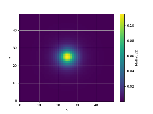
spectractor.extractor.psf.evaluate_moffatgauss2d_jacobian(x, y, amplitude, x_c, y_c, gamma, alpha, eta_gauss, sigma, fixed)[source]

Compute a 2D Moffat+Gauss Jacobian, whose integral is normalised to unity.

Parameters:

x (array_like) – 2D array of pixels \(x\), regularly spaced.
y (array_like) – 2D array of pixels \(y\), regularly spaced.
amplitude (float) – Integral \(A\) of the function.
x_c (float) – X axis center \(x_c\) of the function.
y_c (float) – Y axis center \(y_c\) of the function.
gamma (float) – Width \(\gamma\) of the function.
alpha (float) – Exponent \(\alpha\) of the Moffat function.
eta_gauss (float) – Relative negative amplitude of the Gaussian function.
sigma (float) – Width \(\sigma\) of the Gaussian function.
fixed (array_like) – Array of booleans, with True values for fixed parameters.

Returns:

J – 2D array of the model Jacobian.

Return type:

array_like

Examples

>>> Nx = 50
>>> Ny = 50
>>> yy, xx = np.mgrid[:Ny, :Nx]
>>> amplitude = 10
>>> a = evaluate_moffatgauss2d(xx, yy, amplitude=amplitude, x_c=Nx/2, y_c=Ny/2, gamma=5, alpha=2,
... eta_gauss=-0.1, sigma=1)
>>> J = evaluate_moffatgauss2d_jacobian(xx, yy, amplitude=amplitude, x_c=Nx/2, y_c=Ny/2, gamma=5, alpha=2,
... eta_gauss=-0.1, sigma=1, fixed=np.array([False, False, True, False, False, False, False]))
>>> J.shape
(7, 2500)
>>> J.dtype
dtype('float32')
>>> np.allclose(J[2], 0)
True

spectractor.extractor.psf.load_PSF(psf_type='Moffat', target=None, clip=False)[source]

Load the PSF model with a keyword.

Parameters:

psf_type (str) – PSF model keyword (default: parameters.PSF_TYPE).
target (Target, optional) – The Target instance to make Order0 PSF model (default: None).
clip (bool, optional) – If True, PSF evaluation is clipped between 0 and saturation level (slower) (default: False)

Returns:

psf – An instance of the selected PSF model.

Return type:

PSF

Examples

>>> parameters.VERBOSE = False
>>> load_PSF(psf_type="Gauss", clip=True)  
<....Gauss object at ...>
>>> load_PSF(psf_type="Moffat", clip=True)  
<....Moffat object at ...>
>>> load_PSF(psf_type="MoffatGauss", clip=False)  
<....MoffatGauss object at ...>
>>> from spectractor.extractor.spectrum import Spectrum
>>> spec = Spectrum("./tests/data/reduc_20170530_134_spectrum.fits")  
>>> load_PSF(psf_type="Order0", clip=True, target=spec.target)  
<....Order0 object at ...>

spectractor.extractor.spectroscopy module

class spectractor.extractor.spectroscopy.Line(wavelength, label, atmospheric=False, emission=False, label_pos=[0.007, 0.02], width_bounds=[1, 6], use_for_calibration=False)[source]

Bases: object

Class modeling the emission or absorption lines.

gaussian_model(lambdas, A=1, sigma=2, use_fit=False)[source]

Return a Gaussian model of the spectral line.

Parameters:

lambdas (float, array) – Wavelength array of float in nm
A (float) – Amplitude of the Gaussian (default: +1)
sigma (float) – Standard deviation of the Gaussian (default: 2)
use_fit (bool, optional) – If True, it overrides the previous setting values and use the Gaussian fit made on data, if ti exists.

Returns:

model – The amplitude array of float of the Gaussian model of the line.

Return type:

float, array

Examples

Give lambdas as a float:

>>> l = Line(656.3, atmospheric=False, label='$H\alpha$')
>>> sigma = 2.
>>> model = l.gaussian_model(656.3, A=1, sigma=sigma, use_fit=False)
>>> print(model)
1.0
>>> model = l.gaussian_model(656.3+sigma*np.sqrt(2*np.log(2)), A=1, sigma=sigma, use_fit=False)
>>> print(f"{model:.4f}")
0.5000

Use a fit (for the example we create a mock fit result):

>>> l.fit_lambdas = np.arange(600,700,2)
>>> l.fit_gauss = gauss(l.fit_lambdas, 1e-10, 650, 2.3)
>>> l.fit_fwhm = 2.3*2*np.sqrt(2*np.log(2))
>>> lambdas = np.arange(500,1000,1)
>>> model = l.gaussian_model(lambdas, A=1, sigma=sigma, use_fit=True)
>>> print(model[:5])
[0. 0. 0. 0. 0.]

class spectractor.extractor.spectroscopy.Lines(lines, redshift=0, atmospheric_lines=True, hydrogen_only=False, emission_spectrum=False, orders=[1])[source]

Bases: object

Class gathering all the lines and associated methods.

build_detected_line_table(amplitude_units='', calibration_only=False)[source]

Build the detected line on screen as an Astropy table.

Parameters:

amplitude_units (str, optional) – Units of the line amplitude (default: “”).
calibration_only (bool) – Include only the lines used for calibration if True (default: False).

Returns:

table – Astropy table containing the main line characteristics.

Return type:

Table

Examples

Creation of a mock spectrum with emission and absorption lines

>>> from spectractor.extractor.spectrum import Spectrum, detect_lines
>>> lambdas = np.arange(300,1000,1)
>>> spectrum = 1e4*np.exp(-((lambdas-600)/200)**2)
>>> spectrum += HALPHA.gaussian_model(lambdas, A=5000, sigma=3)
>>> spectrum += HBETA.gaussian_model(lambdas, A=3000, sigma=2)
>>> spectrum += O2_1.gaussian_model(lambdas, A=-3000, sigma=7)
>>> spectrum_err = np.sqrt(spectrum)
>>> spec = Spectrum()
>>> spec.lambdas = lambdas
>>> spec.data = spectrum
>>> spec.err = spectrum_err
>>> fwhm_func = interp1d(lambdas, 0.01 * lambdas)

Detect the lines

>>> lines = Lines([HALPHA, HBETA, O2_1], hydrogen_only=True,
... atmospheric_lines=True, redshift=0, emission_spectrum=True)
>>> global_chisq, res, ws = detect_lines(lines, lambdas, spectrum, spectrum_err, fwhm_func=fwhm_func)
>>> assert(global_chisq < 1.)

Print the result

>>> spec.lines = lines
>>> t = lines.build_detected_line_table()

plot_atomic_lines(ax, color_atomic='g', color_atmospheric='b', fontsize=12, force=False, calibration_only=False)[source]

Over plot the atomic lines as vertical lines, only if they are fitted or with high signal-to-noise ratio, unless force keyword is set to True.

Parameters:

ax (Axes) – An Axes instance on which plot the spectral lines.
color_atomic (str) – Color of the atomic lines (default: ‘g’).
color_atmospheric (str) – Color of the atmospheric lines (default: ‘b’).
fontsize (int) – Font size of the spectral line labels (default: 12).
force (bool) – Force the plot of vertical lines if set to True even if they are not detected (default: False).
calibration_only (bool) – Plot only the lines used for calibration if True (default: False).

Examples

>>> import matplotlib.pyplot as plt
>>> f, ax = plt.subplots(1,1)
>>> ax.set_xlim(300,1000)  
(300..., 1000...)
>>> lines = Lines(HYDROGEN_LINES+ATMOSPHERIC_LINES)
>>> lines.lines[5].fitted = True
>>> lines.lines[5].high_snr = True
>>> lines.lines[-1].fitted = True
>>> lines.lines[-1].high_snr = True
>>> ax = lines.plot_atomic_lines(ax)
>>> if parameters.DISPLAY: plt.show()

(Source code)

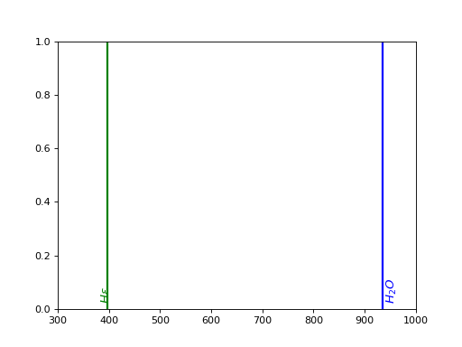
plot_detected_lines(ax=None, calibration_only=False)[source]

Overplot the fitted lines on a spectrum.

Parameters:

ax (Axes) – The Axes instance if needed (default: None).
calibration_only (bool) – Plot only the lines used for calibration if True (default: False).

Examples

Creation of a mock spectrum with emission and absorption lines:

>>> from spectractor.extractor.spectrum import Spectrum, detect_lines
>>> lambdas = np.arange(300,1000,1)
>>> spectrum = 1e4*np.exp(-((lambdas-600)/200)**2)
>>> spectrum += HALPHA.gaussian_model(lambdas, A=5000, sigma=3)
>>> spectrum += HBETA.gaussian_model(lambdas, A=3000, sigma=2)
>>> spectrum += O2_1.gaussian_model(lambdas, A=-3000, sigma=7)
>>> spectrum_err = np.sqrt(spectrum)
>>> spec = Spectrum()
>>> spec.lambdas = lambdas
>>> spec.data = spectrum
>>> spec.err = spectrum_err
>>> fwhm_func = interp1d(lambdas, 0.01 * lambdas)

Detect the lines:

>>> lines = Lines([HALPHA, HBETA, O2_1], hydrogen_only=True,
... atmospheric_lines=True, redshift=0, emission_spectrum=True)
>>> global_chisq, res, ws = detect_lines(lines, lambdas, spectrum, spectrum_err, fwhm_func=fwhm_func)

Plot the result:

>>> spec.lines = lines
>>> fig = plt.figure()
>>> plot_spectrum_simple(plt.gca(), lambdas, spec.data, data_err=spec.err)
>>> lines.plot_detected_lines(plt.gca())
>>> plt.show()

(Source code)

sort_lines()[source]

Sort the lines in increasing order of wavelength, and add the redshift effect.

Returns:: sorted_lines – List of the sorted lines
Return type:: list

Examples

>>> lines = Lines(HYDROGEN_LINES+ATMOSPHERIC_LINES, redshift=0)
>>> sorted_lines = lines.sort_lines()
>>> print([l.wavelength for l in sorted_lines][:5])
[375.0, 377.1, 379.8, 383.5, 388.9]

spectractor.extractor.spectrum module

class spectractor.extractor.spectrum.MultigaussAndBgdFitWorkspace(lines, guess, x, data, err, bounds, bgd_npar, indices, file_name='', verbose=False, plot=False, live_fit=False, truth=None)[source]

Bases: FitWorkspace

jacobian(params, model_input=None)[source]

Generic function to compute the Jacobian matrix of a model, with numerical derivatives.

Parameters:

params (array_like) – The array of model parameters.
model_input (array_like, optional) – A model input as a list with (x, model, model_err) to avoid an additional call to simulate().

Returns:

J – The Jacobian matrix.

Return type:

np.array

reset_x(x)[source]

simulate(*p)[source]

Compute the model prediction given a set of parameters.

Parameters:

p (array_like) – Array of parameters for the computation of the model.

Returns:

x (array_like) – The abscisse of the model prediction.
model (array_like) – The model prediction.
model_err (array_like) – The uncertainty on the model prediction.

Examples

>>> w = FitWorkspace()
>>> p = np.zeros(3)
>>> x, model, model_err = w.simulate(*p)

class spectractor.extractor.spectrum.Spectrum(file_name='', image=None, order=1, target=None, config='', fast_load=False, spectrogram_file_name_override=None, psf_file_name_override=None)[source]

Bases: object

Class used to store information and methods relative to spectra and their extraction.

my_logger

Logging object

Type:: logging

fast_load

If True, only load the spectrum but not the spectrogram.

Type:: bool

units

Units of the spectrum.

Type:: str

lambdas

Spectrum wavelengths in nm.

Type:: array

data

Spectrum amplitude array in self.units units.

Type:: array

err

Spectrum amplitude uncertainties in self.units units.

Type:: array

cov_matrix

Spectrum amplitude covariance matrix between wavelengths in self.units units.

Type:: array

lambdas_binwidths

Bin widths of the wavelength array in nm.

Type:: array

data_next_order

Spectrum amplitude array for next diffraction order in self.units units.

Type:: array

err_next_order

Spectrum amplitude uncertainties for next diffraction order in self.units units.

Type:: array

lambda_ref

Reference wavelength for ADR computations in nm.

Type:: float

order

Index of the diffraction order.

Type:: int

x0

Target position [x,y] in the image in pixels.

Type:: array

psf

PSF instance to model the spectrum PSF.

Type:: PSF

chromatic_psf

ChromaticPSF object that contains data on the PSF shape and evolution in wavelength.

Type:: ChromaticPSF

date_obs

Date of the observation.

Type:: str

airmass

Airmass of the current target.

Type:: float

expo

Exposure time in seconds.

Type:: float

disperser_label

Label of the disperser.

Type:: str

filter_label

Label of the filter.

Type:: str:

rotation_angle

Dispersion axis angle in the image in degrees, positive if anticlockwise.

Type:: float

parallactic_angle

Parallactic angle in degrees.

Type:: float

camera_angle

The North-West axe angle with respect to the camera horizontal axis in degrees.

Type:: float

lines

Lines instance that contains data on the emission or absorption lines to be searched and fitted in the spectrum.

Type:: Lines

header

FITS file header.

Type:: Fits.Header

disperser

Disperser instance that describes the disperser.

Type:: Disperser

target

Target instance that describes the current exposure.

Type:: Target

dec

Declination coordinate of the current exposure in degrees.

Type:: float

hour_angle float: Hour angle coordinate of the current exposure in degrees.

temperature

Outside temperature in Celsius degrees.

Type:: float

pressure

Outside pressure in hPa.

Type:: float

humidity

Outside relative humidity in fraction of one.

Type:: float

throughput

Instrumental throughput of the telescope.

Type:: callable

spectrogram_data

Spectrogram 2D image in image units.

Type:: array

spectrogram_bgd

Estimated 2D background fitted below the spectrogram in image units.

Type:: array

spectrogram_bgd_rms

Estimated 2D background RMS fitted below the spectrogram in image units.

Type:: array

spectrogram_err

Estimated 2D background uncertainty fitted below the spectrogram in image units.

Type:: array

spectrogram_fit

Best fitting model of the spectrogram in image units.

Type:: array

spectrogram_residuals

Residuals between the spectrogram data and the best fitting model of the spectrogram in image units.

Type:: array

spectrogram_flat

Flat array for the spectrogram with average=1.

Type:: array

spectrogram_starfield

Star field simulation array for the spectrogram in ADU/s.

Type:: array

spectrogram_mask

Boolean mask array to flag the defects.

Type:: array

spectrogram_x0

Relative position of the target in the spectrogram array along the x axis.

Type:: float

spectrogram_y0

Relative position of the target in the spectrogram array along the y axis.

Type:: float

spectrogram_xmin

Left index of the spectrogram crop in the image.

Type:: int

spectrogram_xmax

Right index of the spectrogram crop in the image.

Type:: int

spectrogram_ymin

Bottom index of the spectrogram crop in the image.

Type:: int

spectrogram_ymax

Top index of the spectrogram crop in the image.

Type:: int

spectrogram_deg

Degree of the polynomial functions to model wavelength evolutions of the PSF parameters.

Type:: int

spectrogram_saturation

Level of saturation in the spectrogram in image units.

Type:: float

spectrogram_Nx

Size of the spectrogram along the x axis.

Type:: int

spectrogram_Ny

Size of the spectrogram along the y axis.

Type:: int

compute_disp_axis_in_spectrogram(shift_x, shift_y, angle)[source]

Compute the dispersion axis position in a spectrogram. Origin is the order 0 centroid.

Parameters:

shift_x (float) – Shift in the x axis direction for order 0 position in pixel.
shift_y (float) – Shift in the y axis direction for order 0 position in pixel.
angle (float) – Main dispersion axis angle in degrees.

Returns:

Dx (array_like) – Position array along x axis of spectrogram
Dy_disp_axis (array_like) – Dispersion axis position along y axis of spectrogram with respect to Dx.

Examples

>>> s = Spectrum("./tests/data/reduc_20170530_134_spectrum.fits")
>>> Dx, Dy_disp_axis = s.compute_disp_axis_in_spectrogram(0, 0, 0)
>>> Dx[0] == -s.spectrogram_x0
True
>>> Dy_disp_axis[:4]
array([0., 0., 0., 0.])

compute_dispersion_in_spectrogram(lambdas, D, shift_x, shift_y, angle, with_adr=True, order=1)[source]

Compute the dispersion relation in a spectrogram, using grating dispersion model and ADR, for a given diffraction order. Origin is the order 0 centroid.

Parameters:

lambdas (array_like) – Wavelength array for the given diffraction order.
D (float) – The distance between the CCD and the disperser in mm.
shift_x (float) – Shift in the x axis direction for order 0 position in pixel.
shift_y (float) – Shift in the y axis direction for order 0 position in pixel.
angle (float) – Main dispersion axis angle in degrees.
with_adr (bool, optional) – If True, add ADR effect to grating dispersion model (default: True).
order (int, optional) – Diffraction order (default: 1).

Returns:

dispersion_law – Complex array coding the 2D dispersion relation in the spectrogram for the given diffraction order.

Return type:

array_like

Examples

>>> s = Spectrum("./tests/data/reduc_20170530_134_spectrum.fits")
>>> s.x0 = [743, 683]
>>> s.spectrogram_x0 = -280
>>> lambdas = s.compute_lambdas_in_spectrogram(58, 0, 0, 0)
>>> lambdas[:4]  
array([334.874..., 336.022..., 337.170..., 338.318...])
>>> dispersion_law = s.compute_dispersion_in_spectrogram(lambdas, 58, 0, 0, 0, order=1)
>>> dispersion_law[:4]  
array([280.0... +1.0...j, 281.0...+1.0...j,
       282.0...+1.0...j, 283.0... +1.0...j])
>>> dispersion_law_order2 = s.compute_dispersion_in_spectrogram(lambdas, 58, 0, 0, 0, order=2)
>>> dispersion_law_order2[:4]  
array([573.6...+1.0...j, 575.8...+1.0...j,
       577.9...+1.0...j, 580.0...+1.0...j])

compute_lambdas_in_spectrogram(D, shift_x, shift_y, angle, niter=3, with_adr=True, order=1)[source]

Compute the dispersion relation in a spectrogram, using grating dispersion model and ADR, for a given diffraction order. Origin is the order 0 centroid.

Parameters:

D (float) – The distance between the CCD and the disperser in mm.
shift_x (float) – Shift in the x axis direction for order 0 position in pixel.
shift_y (float) – Shift in the y axis direction for order 0 position in pixel.
angle (float) – Main dispersion axis angle in degrees.
niter (int, optional) – Number of iterations to compute ADR (default: 3).
with_adr (bool, optional) – If True, add ADR effect to grating dispersion model (default: True).
order (int, optional) – Diffraction order (default: 1).

Returns:

lambdas – Wavelength array for the given diffraction order.

Return type:

array_like

Examples

>>> s = Spectrum("./tests/data/reduc_20170530_134_spectrum.fits")
>>> s.x0 = [743, 683]
>>> s.spectrogram_x0 = -280
>>> lambdas = s.compute_lambdas_in_spectrogram(58, 0, 0, 0)
>>> lambdas[:4]  
array([334.874..., 336.022..., 337.170..., 338.318...])
>>> lambdas_order2 = s.compute_lambdas_in_spectrogram(58, 0, 0, 0, order=2)
>>> lambdas_order2[:4]  
array([175.248..., 175.661..., 176.088..., 176.527...])

convert_from_ADUrate_to_flam()[source]

Convert units from ADU/s to erg/s/cm^2/nm. The SED is supposed to be in flam units ie erg/s/cm^2/nm

Examples

>>> s = Spectrum(file_name='tests/data/reduc_20170605_028_spectrum.fits', config="./config/ctio.ini")
>>> s.convert_from_ADUrate_to_flam()

convert_from_flam_to_ADUrate()[source]

Convert units from erg/s/cm^2/nm to ADU/s. The SED is supposed to be in flam units ie erg/s/cm^2/nm

Examples

>>> s = Spectrum(file_name='tests/data/reduc_20170605_028_spectrum.fits', config="./config/ctio.ini")
>>> s.convert_from_flam_to_ADUrate()

load_chromatic_psf(input_file_name)[source]

OBSOLETE: Load the spectrum from a fits file (data, error and wavelengths).

Parameters:: input_file_name (str) – Path to the input fits file

Examples

>>> s = Spectrum('./tests/data/reduc_20170530_134_spectrum.fits')
>>> print(s.chromatic_psf.table)  
     lambdas               Dx        ...

load_filter()[source]

Load filter properties and set relevant LAMBDA_MIN and LAMBDA_MAX values.

Examples

>>> s = Spectrum(config="./config/ctio.ini")
>>> s.filter_label = 'FGB37'
>>> _ = s.load_filter()

load_spectrogram(input_file_name)[source]

OBSOLETE: Load the spectrum from a fits file (data, error and wavelengths).

Parameters:: input_file_name (str) – Path to the input fits file

Examples

>>> s = Spectrum(config="./config/ctio.ini")
>>> s.load_spectrum('tests/data/reduc_20170605_028_spectrum.fits')

load_spectrum(input_file_name, spectrogram_file_name_override=None, psf_file_name_override=None, fast_load=False)[source]

Load the spectrum from a fits file (data, error and wavelengths).

Parameters:

input_file_name (str) – Path to the input fits file
spectrogram_file_name_override (str) – Manually specify a path to the spectrogram file.
psf_file_name_override (str) – Manually specify a path to the psf file.
fast_load (bool, optional) – If True, only the spectrum is loaded (not the PSF nor the spectrogram data) (default: False).

Examples

Latest Spectractor output format: do not provide a config file (parameters are loaded from file header)

>>> from spectractor import parameters
>>> s = Spectrum(config="")
>>> s.load_spectrum('tests/data/reduc_20170530_134_spectrum.fits')

Spectractor output format older than version <=2.3: must give the config file

>>> parameters.VERBOSE = False
>>> s = Spectrum(config="./config/ctio.ini")
>>> s.load_spectrum('tests/data/reduc_20170605_028_spectrum.fits')
>>> print(s.units)
erg/s/cm$^2$/nm

load_spectrum_latest(input_file_name)[source]

Load the spectrum from a FITS file (data, error and wavelengths) from Spectrum files generated with Spectractor software above or equal 2.4 version. The parameters are loaded via the FITS file header and overwrites those loaded via the config file.

Parameters:: input_file_name (str) – Path to the input fits file

Examples

>>> s = Spectrum(config="")
>>> s.load_spectrum('tests/data/reduc_20170530_134_spectrum.fits')
>>> print(s.units)
erg/s/cm$^2$/nm

load_spectrum_older_24(input_file_name, spectrogram_file_name_override=None, psf_file_name_override=None, fast_load=False)[source]

Load the spectrum from a FITS file (data, error and wavelengths) from Spectrum files generated with Spectractor software strictly older than 2.4 version. The parameters must be loaded via the config files.

Parameters:

input_file_name (str) – Path to the input fits file
spectrogram_file_name_override (str) – Manually specify a path to the spectrogram file.
psf_file_name_override (str) – Manually specify a path to the psf file.
fast_load (bool, optional) – If True, only the spectrum is loaded (not the PSF nor the spectrogram data) (default: False).

Examples

>>> s = Spectrum(config="./config/ctio.ini")
>>> s.load_spectrum('tests/data/reduc_20170605_028_spectrum.fits')
>>> print(s.units)
erg/s/cm$^2$/nm

plot_spectrogram(ax=None, scale='lin', title='', units='Image units', plot_stats=False, target_pixcoords=None, vmin=None, vmax=None, figsize=[9.3, 8], aspect=None, cmap=None, cax=None)[source]

Plot spectrogram.

Parameters:

ax (Axes, optional) – Axes instance (default: None).
scale (str) – Scaling of the image (choose between: lin, log or log10) (default: lin)
title (str) – Title of the image (default: “”)
units (str) – Units of the image to be written in the color bar label (default: “Image units”)
cmap (colormap) – Color map label (default: None)
target_pixcoords (array_like, optional) – 2D array giving the (x,y) coordinates of the targets on the image: add a scatter plot (default: None)
vmin (float) – Minimum value of the image (default: None)
vmax (float) – Maximum value of the image (default: None)
aspect (str) – Aspect keyword to be passed to imshow (default: None)
cax (Axes, optional) – Color bar axes if necessary (default: None).
figsize (tuple) – Figure size (default: [9.3, 8]).
plot_stats (bool) – If True, plot the uncertainty map instead of the spectrogram (default: False).

Examples

>>> s = Spectrum(file_name='tests/data/reduc_20170530_134_spectrum.fits')
>>> s.plot_spectrogram()
>>> if parameters.DISPLAY: plt.show()

(Source code)

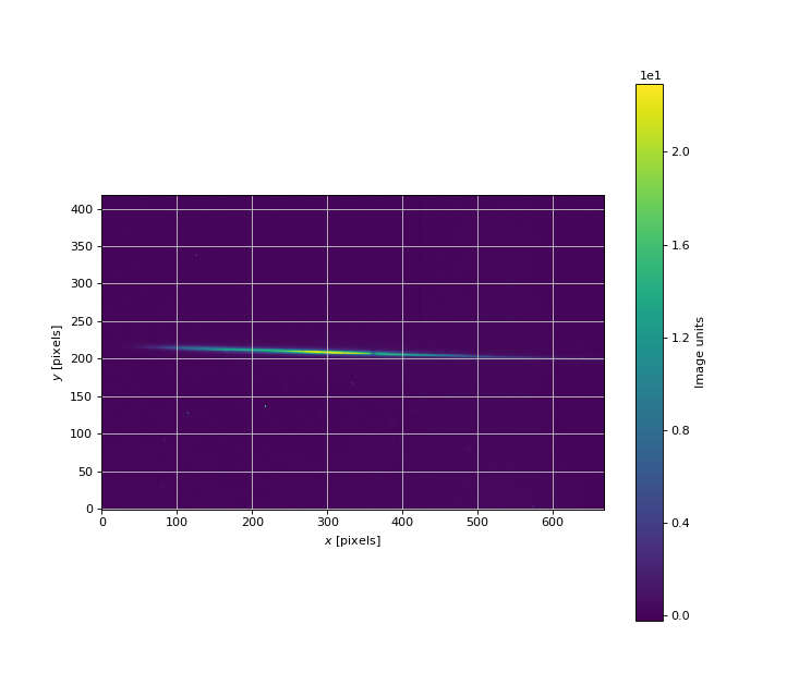
plot_spectrum(ax=None, xlim=None, live_fit=False, label='', force_lines=False, calibration_only=False)[source]

Plot spectrum with emission and absorption lines.

Parameters:

ax (Axes, optional) – Axes instance (default: None).
label (str) – Label for the legend (default: ‘’).
xlim (list, optional) – List of minimum and maximum abscisses (default: None)
live_fit (bool, optional) – If True the spectrum is plotted in live during the fitting procedures (default: False).
force_lines (bool) – Force the over plot of vertical lines for atomic lines if set to True (default: False).
calibration_only (bool) – Plot only the lines used for calibration if True (default: False).

Examples

>>> s = Spectrum(file_name='tests/data/reduc_20170530_134_spectrum.fits')
>>> s.plot_spectrum(xlim=[500,900], live_fit=False, force_lines=True)

plot_spectrum_summary(xlim=None, figsize=(12, 12), save_as='')[source]

Plot spectrum with emission and absorption lines.

Parameters:

xlim (list, optional) – List of minimum and maximum abscisses (default: None).
figsize (tuple) – Figure size (default: (12, 12)).
save_as (str, optional) – Path to save the figure to, if specified.

Examples

>>> s = Spectrum(file_name='tests/data/reduc_20170530_134_spectrum.fits')
>>> s.plot_spectrum_summary()

save_spectrogram(output_file_name, overwrite=False)[source]

OBOSOLETE: save the spectrogram into a fits file (data, error and background).

Parameters:

output_file_name (str) – Path of the output fits file.
overwrite (bool, optional) – If True overwrite the output file if needed (default: False).

Examples

save_spectrum(output_file_name, overwrite=False)[source]

Save the spectrum into a fits file (data, error and wavelengths).

Parameters:

output_file_name (str) – Path of the output fits file.
overwrite (bool) – If True overwrite the output file if needed (default: False).

Examples

>>> import os
>>> s = Spectrum(file_name='tests/data/reduc_20170530_134_spectrum.fits')
>>> s.save_spectrum('./tests/test.fits')

Overwrite previous file: >>> s.save_spectrum(‘./tests/test.fits’, overwrite=True)

spectractor.extractor.spectrum.calibrate_spectrum(spectrum, with_adr=False, niter=5, grid_search=False)[source]

Convert pixels into wavelengths given the position of the order 0, the data for the spectrum, the properties of the disperser. Fit the absorption (and eventually the emission) lines to perform a second calibration of the distance between the CCD and the disperser. The number of fitting steps is limited to 30.

Finally convert the spectrum amplitude from ADU rate to erg/s/cm2/nm.

Parameters:

spectrum (Spectrum) – Spectrum object to calibrate
with_adr (bool, optional) – If True, the ADR longitudinal shift is subtracted to distances. Must be False if the spectrum has already been decontaminated from ADR (default: False).
niter (int, optional) – Number of iterations for ADR accurate evaluation (default: 5).

Returns:

lambdas – The new wavelength array in nm.

Return type:

array_like

Examples

>>> spectrum = Spectrum('tests/data/reduc_20170530_134_spectrum.fits', config="")
>>> parameters.LAMBDA_MIN = 350
>>> parameters.LAMBDA_MAX = 800
>>> parameters.DEBUG = True
>>> parameters.PIXSHIFT_PRIOR = 2
>>> parameters.DISTANCE2CCD_ERR = 0.05
>>> lambdas = calibrate_spectrum(spectrum, with_adr=True, grid_search=True)
>>> spectrum.plot_spectrum()

spectractor.extractor.spectrum.detect_lines(lines, lambdas, spec, spec_err=None, cov_matrix=None, fwhm_func=None, snr_minlevel=3, ax=None, calibration_lines_only=False, xlim=(300, 1100))[source]

Detect and fit the lines in a spectrum. The method is to look at maxima or minima around emission or absorption tabulated lines, and to select surrounding pixels to fit a (positive or negative) gaussian and a polynomial background. If several regions overlap, a multi-gaussian fit is performed above a common polynomial background. The mean global shift (in nm) between the detected and tabulated lines is returned, considering only the lines with a signal-to-noise ratio above a threshold. The order of the polynomial background is set in parameters.py with CALIB_BGD_ORDER.

Parameters:

lines (Lines) – The Lines object containing the line characteristics
lambdas (float array) – The wavelength array (in nm)
spec (float array) – The spectrum amplitude array
spec_err (float array, optional) – The spectrum amplitude uncertainty array (default: None)
cov_matrix (float array, optional) – The spectrum amplitude 2D covariance matrix array (default: None)
fwhm_func (callable, optional) – The fwhm of the cross spectrum to reset CALIB_PEAK_WIDTH parameter as a function of lambda (default: None)
snr_minlevel (float) – The minimum signal over noise ratio to consider using a fitted line in the computation of the mean shift output and to print it in the outpur table (default: 3)
ax (Axes, optional) – An Axes instance to over plot the result of the fit (default: None).
calibration_lines_only (bool, optional) – If True, try to detect only the lines with use_for_calibration attributes set True.
xlim (array, optional) – (min, max) list limiting the wavelength interval where to detect spectral lines (default: (parameters.LAMBDA_MIN, parameters.LAMBDA_MAX))

Returns:

shift – The mean shift (in nm) between the detected and tabulated lines

Return type:

float

Examples

Creation of a mock spectrum with emission and absorption lines:

>>> import numpy as np
>>> from spectractor.extractor.spectroscopy import Lines, HALPHA, HBETA, O2_1
>>> lambdas = np.arange(300,1000,1)
>>> spectrum = 1e4*np.exp(-((lambdas-600)/200)**2)
>>> spectrum += HALPHA.gaussian_model(lambdas, A=5000, sigma=3)
>>> spectrum += HBETA.gaussian_model(lambdas, A=3000, sigma=2)
>>> spectrum += O2_1.gaussian_model(lambdas, A=-3000, sigma=7)
>>> spectrum_err = np.sqrt(spectrum)
>>> cov = np.diag(spectrum_err)
>>> spectrum = np.random.poisson(spectrum)
>>> spec = Spectrum()
>>> spec.lambdas = lambdas
>>> spec.data = spectrum
>>> spec.err = spectrum_err
>>> fwhm_func = interp1d(lambdas, 0.01 * lambdas)

Detect the lines:

>>> lines = Lines([HALPHA, HBETA, O2_1], hydrogen_only=True,
... atmospheric_lines=True, redshift=0, emission_spectrum=True)
>>> global_chisq, _, _ = detect_lines(lines, lambdas, spectrum, spectrum_err, cov, fwhm_func=fwhm_func)

Plot the result:

>>> import matplotlib.pyplot as plt
>>> spec.lines = lines
>>> fig = plt.figure()
>>> plot_spectrum_simple(plt.gca(), lambdas, spec.data, data_err=spec.err)
>>> lines.plot_detected_lines(plt.gca())
>>> if parameters.DISPLAY: plt.show()

spectractor.extractor.spectrum.run_multigaussandbgd_minimisation(w)[source]

spectractor.extractor.targets module

class spectractor.extractor.targets.ArcLamp(label, verbose=False)[source]

Bases: Target

load()[source]

class spectractor.extractor.targets.Led(label, verbose=False)[source]

Bases: Target

load()[source]

class spectractor.extractor.targets.Monochromator(label, verbose=False)[source]

Bases: Target

load()[source]

class spectractor.extractor.targets.Star(label, verbose=False)[source]

Bases: Target

build_sed(index=0)[source]

Interpolate the database reference spectra and return self.sed as a function of the wavelength.

Parameters:: index (int) – Index of the spectrum stored in the self.spectra list

Examples

>>> s = Star('HD111980')
>>> s.build_sed(index=0)
>>> s.sed(550)
array(1.67508011e-11)

get_radec_position_after_pm(table_coordinates, date_obs='J2000', date_reference='J2000')[source]

load()[source]

Load the coordinates of the target.

Examples

>>> parameters.VERBOSE = True
>>> s = Star('PNG321.0+3.9')
>>> print(s.radec_position.dec)  
-54d18m07...s
>>> print(s.redshift)  
-0.00021...
>>> s = Star('eta dor')
>>> print(s.radec_position.dec)  
-66d02m22...s
>>> s = Star('mu.col')
>>> print(s.radec_position.dec)  
-32d18m23...s

load_calspec()[source]

load_emission_spectrum(hydrogen_only_flag)[source]

load_gaia()[source]

Load the spectrum from the Gaia database.

Examples

>>> s = Star('HD111980')
>>> s.load_gaia()
>>> s.plot_spectra()

load_ned()[source]

Load the spectrum from NED database.

Examples

>>> s = Star('3C273')
>>> s.load_ned()
>>> s.plot_spectra()

load_spectra()[source]

Load reference spectra from getCalspec database or NED database.

If the object redshift is >0.2, the LAMBDA_MIN and LAMBDA_MAX parameters are redshifted accordingly.

Examples

>>> s = Star('HD111980')
>>> print(s.spectra[0][:4])
[2.2839e-13 2.0263e-13 2.0889e-13 2.3928e-13]
>>> print(f'{parameters.LAMBDA_MIN:.1f}, {parameters.LAMBDA_MAX:.1f}')
300.0, 1100.0
>>> print(s.spectra[0][:4])
[2.2839e-13 2.0263e-13 2.0889e-13 2.3928e-13]

plot_spectra()[source]

Plot the spectra stored in the self.spectra list.

Examples

>>> s = Star('HD111980')
>>> s.plot_spectra()

class spectractor.extractor.targets.Target(label, verbose=False)[source]: Bases: object

spectractor.extractor.targets.load_target(label, verbose=False)[source]

Load the target properties according to the type set by parameters.OBS_OBJECT_TYPE.

Currently, the type can be either “STAR”, “HG-AR” or “MONOCHROMATOR”. The label parameter gives the name of the source and allows to load its specific properties.

Parameters:

label (str) – The label of the target.
verbose (bool, optional) – If True, more verbosity (default: False).

Examples

>>> parameters.OBS_OBJECT_TYPE = "STAR"
>>> t = load_target("HD111980", verbose=False)
>>> print(t.label)
HD111980
>>> print(t.radec_position.dec)  
-18d31m...s
>>> parameters.OBS_OBJECT_TYPE = "MONOCHROMATOR"
>>> t = load_target("XX", verbose=False)
>>> print(t.label)
XX
>>> parameters.OBS_OBJECT_TYPE = "HG-AR"
>>> t = load_target("XX", verbose=False)
>>> print([line.wavelength for line in t.lines.lines][:5])
[253.652, 296.728, 302.15, 313.155, 334.148]

spectractor.extractor.targets.patchSimbadURL(simbad)[source]

Monkeypatch the URL that Simbad is using to force it to use https.

This is necessary to make the tests on github actions work, because for some reason it wasn’t automatically upgrading to https otherwise.

spectractor.extractor package

Submodules

spectractor.extractor.chromaticpsf module

spectractor.extractor.dispersers module

spectractor.extractor.extractor module

spectractor.extractor.images module

spectractor.extractor.psf module

spectractor.extractor.spectroscopy module

spectractor.extractor.spectrum module

spectractor.extractor.targets module

Module contents