spectractor package

Subpackages

Submodules

spectractor.config module

spectractor.config.apply_rebinning_to_parameters()[source]

Divide or multiply original parameters by parameters.CCD_REBIN to set them correctly in the case of an image rebinning.

Examples

>>> parameters.PIXWIDTH_SIGNAL = 40
>>> parameters.CCD_PIXEL2MM = 10
>>> parameters.CCD_REBIN = 2
>>> apply_rebinning_to_parameters()
>>> parameters.PIXWIDTH_SIGNAL
20
>>> parameters.CCD_PIXEL2MM
20

spectractor.config.from_config_to_dict(path)[source]

Convert config file keywords into dictionnary.

Parameters:: path (str) – The path to the config file.

Examples

>>> mypath = os.path.dirname(__file__)
>>> out = from_config_to_dict(os.path.join(mypath, "../config/", "default.ini"))
>>> assert type(out) == dict

spectractor.config.from_config_to_parameters(path)[source]

Convert config file keywords into spectractor.parameters parameters.

Parameters:: path (str) – The path to the config file.

Examples

>>> mypath = os.path.dirname(__file__)
>>> from_config_to_parameters(os.path.join(mypath, parameters.CONFIG_DIR, "default.ini"))
>>> assert parameters.OBS_NAME == "DEFAULT"

spectractor.config.load_config(config_filename, rebin=True)[source]

Load configuration parameters from a .ini config file.

Parameters:

config_filename (str) – The path to the config file.
rebin (bool, optional) – If True, the parameters.REBIN parameter is used and every parameters are changed to comply with the REBIN value. If False, the parameters.REBIN parameter is skipped and set to 1.

Examples

>>> parameters.VERBOSE = True
>>> load_config("./config/ctio.ini")
>>> assert parameters.OBS_NAME == "CTIO"

spectractor.config.set_logger(logger)[source]

Logger function for all classes.

Parameters:: logger (str) – Name of the class, usually self.__class__.__name__
Returns:: my_logger – Logging object
Return type:: logging

Examples

>>> class Test:
...     def __init__(self):
...         self.my_logger = set_logger(self.__class__.__name__)
...     def log(self):
...         self.my_logger.info('This info test function works.')
...         self.my_logger.debug('This debug test function works.')
...         self.my_logger.warning('This warning test function works.')
>>> from spectractor import parameters
>>> parameters.VERBOSE = True
>>> parameters.DEBUG = True
>>> test = Test()
>>> test.log()

spectractor.config.update_derived_parameters()[source]

spectractor.logbook module

class spectractor.logbook.LogBook(logbook='./tests/data/ctiofulllogbook_jun2017_v5.csv')[source]

Bases: object

Class to load_image and analyse observation logbook csv files.

plot_columns_vs_date(column_names)[source]

Plot of the column property with respect to the dates.

Parameters:: column_names (list, str) – List of column names to plot versus time from the log book.

Examples

>>> logbook = LogBook('./tests/data/ctiofulllogbook_jun2017_v5.csv')
>>> logbook.plot_columns_vs_date(['seeing'])
>>> logbook.plot_columns_vs_date(['P', 'T'])

search_for_image(filename)[source]

Look for an image file name in the logbook and load_image properties:

Obj-posXpix and Obj-posYpix: the [x0,y0] guessed pixel position in the image
Dx and Dy: the x and y windows in pixel to search for the target; set XWINDOW and YWINDOW variables in parameters.py
object: the name of the target

Parameters:

filename (str) – the fits image file name (not the path, only the file name.)

Returns:

disperser_label (str) – the name of the disperser
target (str) – the name of the target
xpos (int) – the x position of the target (in pixel)
ypos (int) – the y position of the target (in pixel)

Examples

>>> logbook = LogBook('./tests/data/ctiofulllogbook_jun2017_v5.csv')
>>> disperser_label, target, xpos, ypos = logbook.search_for_image("unknown_file.fits")
>>> print(disperser_label, target, xpos, ypos)
None None None None
>>> disperser_label, target, xpos, ypos = logbook.search_for_image("reduc_20170605_028.fits")
>>> print(disperser_label, target, xpos, ypos)
HoloPhAg PNG321.0+3.9 814 585
>>> disperser_label, target, xpos, ypos = logbook.search_for_image("reduc_20170608_119.fits")
>>> print(disperser_label, target, xpos, ypos)
None HD205905 None None
>>> disperser_label, target, xpos, ypos = logbook.search_for_image("reduc_20170630_001.fits")
>>> print(disperser_label, target, xpos, ypos)
None bias None None

spectractor.parameters module

spectractor.tools module

class spectractor.tools.NumpyArrayEncoder(*, skipkeys=False, ensure_ascii=True, check_circular=True, allow_nan=True, sort_keys=False, indent=None, separators=None, default=None)[source]

Bases: JSONEncoder

default(obj)[source]

Implement this method in a subclass such that it returns a serializable object for o, or calls the base implementation (to raise a TypeError).

For example, to support arbitrary iterators, you could implement default like this:

def default(self, o):
    try:
        iterable = iter(o)
    except TypeError:
        pass
    else:
        return list(iterable)
    # Let the base class default method raise the TypeError
    return JSONEncoder.default(self, o)

spectractor.tools.cholesky_solve(A, B)[source]

Solve the system A @ X = B using Cholesky factorisation.

Parameters:

A (np.ndarray) – Matrix
B (np.ndarray) – Vector

Returns:

X – Solution

Return type:

np.ndarray

Examples

>>> N = 1000
>>> A = np.tri(N).T @ np.tri(N)
>>> B = np.arange(N)
>>> cov_matrix = np.linalg.inv(A)
>>> X = cov_matrix @ B
>>> X2 = cholesky_solve(A, B)
>>> assert np.all(np.abs(X - X2)<1e-10)

spectractor.tools.clean_target_spikes(data, saturation)[source]

spectractor.tools.compute_correlation_matrix(cov)[source]

Compute correlation matrix from a covariance matrix.

Parameters:: cov (np.ndarray) – Covariance matrix.
Returns:: rho – Correlation matrix.
Return type:: np.ndarray

Examples

>>> cov = np.array([[4, 1], [1, 16]])
>>> compute_correlation_matrix(cov)
array([[1.   , 0.125],
       [0.125, 1.   ]])

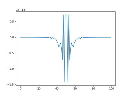
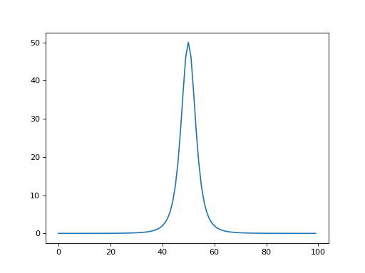
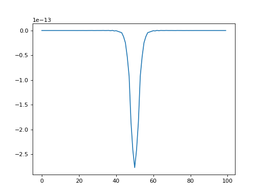
spectractor.tools.compute_fwhm(x, y, minimum=0, center=None, full_output=False, epsilon=0.001)[source]

Compute the full width half maximum of y(x) curve, using an interpolation of the data points and dichotomie method.

Parameters:

x (array_like) – The abscisse array.
y (array_like) – The function array.
minimum (float, optional) – The minimum reference from which to compyte half the height (default: 0).
center (float, optional) – The center of the curve. If None, the weighted averageof the y(x) distribution is computed (default: None).
full_output (bool, optional) – If True, half maximum, the edges of the curve and the curve center are given in output (default: False).
epsilon (float, optional) – Dichotomie algorithm stop if difference is smaller than epsilon (default: 1e-3).

Returns:

FWHM (float) – The full width half maximum of the curve.
half (float, optional) – The half maximum value. Only if full_output=True.
center (float, optional) – The y(x) center value. Only if full_output=True.
left_edge (float, optional) – The left_edge value at half maximum. Only if full_output=True.
right_edge (float, optional) – The right_edge value at half maximum. Only if full_output=True.

Examples

Gaussian example

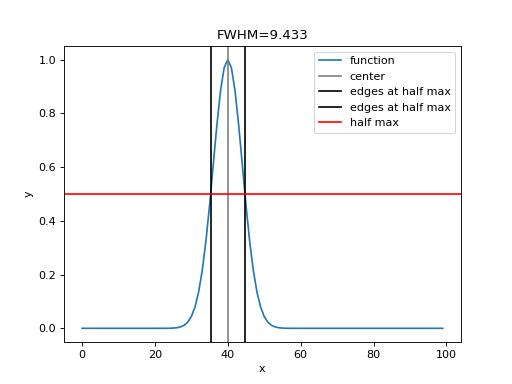
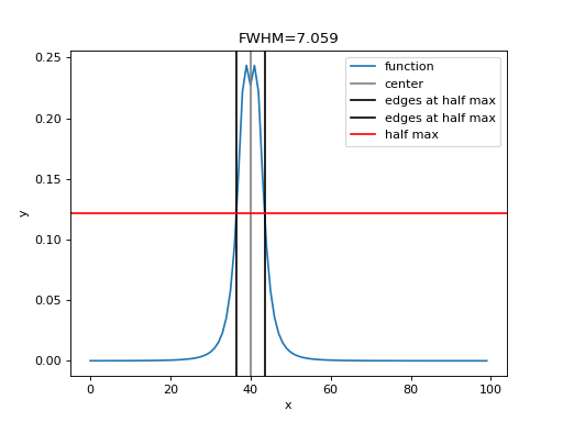
>>> x = np.arange(0, 100, 1)
>>> stddev = 4
>>> middle = 40
>>> psf = gauss(x, 1, middle, stddev)
>>> fwhm, half, center, a, b = compute_fwhm(x, psf, full_output=True)
>>> print(f"{fwhm:.4f} {2.355*stddev:.4f} {center:.4f}")
9.4329 9.4200 40.0000

(Source code)

Defocused PSF example

>>> from spectractor.extractor.psf import MoffatGauss
>>> p = [2,40,40,4,2,-0.4,1,10]
>>> psf = MoffatGauss(p)
>>> fwhm, half, center, a, b = compute_fwhm(x, psf.evaluate(x), full_output=True)

(Source code)

spectractor.tools.compute_integral(x, y, bounds=None)[source]

Compute the integral of an y(x) curve. The curve is interpolated and extrapolated with cubic splines. If not provided, bounds are set to the x array edges.

Parameters:

x (array_like) – The abscisse array.
y (array_like) – The function array.
bounds (array_like, optional) – The bounds of the integral. If None, the edges of thex array are taken (default bounds=None).

Returns:

result – The integral of the PSF model.

Return type:

float

Examples

Gaussian example

>>> x = np.arange(0, 100, 1)
>>> stddev = 4
>>> middle = 40
>>> psf = gauss(x, 1/(stddev*np.sqrt(2*np.pi)), middle, stddev)
>>> integral = compute_integral(x, psf)
>>> print(f"{integral:.6f}")
1.000000

Defocused PSF example

>>> from spectractor.extractor.psf import MoffatGauss
>>> p = [2,30,30,4,2,-0.5,1,10]
>>> psf = MoffatGauss(p)
>>> integral = compute_integral(x, psf.evaluate(x))
>>> assert np.isclose(integral, p[0], atol=1e-2)

spectractor.tools.detect_peaks(image)[source]

Takes an image and detect the peaks using the local maximum filter. Returns a boolean mask of the peaks (i.e. 1 when the pixel’s value is the neighborhood maximum, 0 otherwise). Only positive peaks are detected (take absolute value or negative value of the image to detect the negative ones).

Parameters:: image (array_like) – The image 2D array.
Returns:: detected_peaks – Boolean maskof the peaks.
Return type:: array_like

Examples

>>> im = np.zeros((50,50))
>>> im[4,6] = 2
>>> im[10,20] = -3
>>> im[49,49] = 1
>>> detected_peaks = detect_peaks(im)

spectractor.tools.dichotomie(f, a, b, epsilon)[source]

Dichotomie method to find a function root.

Parameters:

f (callable) – The function
a (float) – Left bound to the expected root
b (float) – Right bound to the expected root
epsilon (float) – Precision

Returns:

root – The root of the function.

Return type:

float

Examples

Search for the Gaussian FWHM:

>>> p = [1,0,1]
>>> xx = np.arange(-10,10,0.1)
>>> PSF = gauss(xx, *p)
>>> def eq(x):
...     return np.interp(x, xx, PSF) - 0.5
>>> root = dichotomie(eq, 0, 10, 1e-6)
>>> assert np.isclose(2*root, 2.355*p[2], 1e-3)

spectractor.tools.ensure_dir(directory_name)[source]

Ensure that directory_name directory exists. If not, create it.

Parameters:: directory_name (str) – The directory name.

Examples

>>> ensure_dir('tests')
>>> os.path.exists('tests')
True
>>> ensure_dir('tests/mytest')
>>> os.path.exists('tests/mytest')
True
>>> os.rmdir('./tests/mytest')

spectractor.tools.fftconvolve_gaussian(array, reso)[source]

Convolve an 1D or 2D array with a Gaussian profile of given standard deviation.

Parameters:

array (array) – The array to convolve.
reso (float) – The standard deviation of the Gaussian profile.

Returns:

convolved – The convolved array, same size and shape as input.

Return type:

array

Examples

>>> array = np.ones(100)
>>> output = fftconvolve_gaussian(array, 3)
>>> print(output[:3])
[0.5        0.63114657 0.74850168]
>>> array = np.ones((100, 100))
>>> output = fftconvolve_gaussian(array, 3)
>>> print(output[0][:3])
[0.5        0.63114657 0.74850168]
>>> array = np.ones((100, 100, 100))
>>> output = fftconvolve_gaussian(array, 3)

spectractor.tools.filter_stars_from_bgd(data, margin_cut=1)[source]

spectractor.tools.find_nearest(array, value)[source]

Find the nearest index and value in an array.

Parameters:

array (array) – The array to inspect.
value (float) – The value to look for.

Returns:

index (int) – The array index of the nearest value close to value
val (float) – The value fo the array at index.

Examples

>>> x = np.arange(0.,10.)
>>> idx, val = find_nearest(x, 3.3)
>>> print(idx, val)
3 3.0

spectractor.tools.fit_gauss(x, y, guess=[10, 1000, 1], bounds=(-inf, inf), sigma=None)[source]

Fit a Gaussian profile to data, using curve_fit. The mean guess value of the Gaussian must not be far from the truth values. Boundaries helps a lot also.

Parameters:

x (np.array) – The x data values.
y (np.array) – The y data values.
guess (list, [amplitude, mean, sigma], optional) – List of first guessed values for the Gaussian fit (default: [10, 1000, 1]).
bounds (list, optional) – List of boundaries for the parameters [[minima],[maxima]] (default: (-np.inf, np.inf)).
sigma (np.array, optional) – The y data uncertainties.

Returns:

popt (list) – Best fitting parameters of curve_fit.
pcov (list) – Best fitting parameters covariance matrix from curve_fit.

Examples

>>> import numpy as np
>>> import matplotlib.pyplot as plt
>>> x = np.arange(600.,700.,2)
>>> p = [10, 650, 10]
>>> y = gauss(x, *p)
>>> y_err = np.ones_like(y)
>>> print(y[25])
10.0
>>> guess = (2,630,2)
>>> popt, pcov = fit_gauss(x, y, guess=guess, bounds=((1,600,1),(100,700,100)), sigma=y_err)

spectractor.tools.fit_gauss2d_outlier_removal(x, y, z, sigma=3.0, niter=3, guess=None, bounds=None, circular=False)[source]

Fit an astropy Gaussian 2D model with parameters : amplitude, x_mean, y_mean, x_stddev, y_stddev, theta using outlier removal methods.

Parameters:

x (np.array) – 2D array of the x coordinates from meshgrid.
y (np.array) – 2D array of the y coordinates from meshgrid.
z (np.array) – the 2D array image.
sigma (float) – value of sigma for the sigma rejection of outliers (default: 3)
niter (int) – maximum number of iterations for the outlier detection (default: 3)
guess (list, optional) – List containing a first guess for the PSF parameters (default: None).
bounds (list, optional) – 2D list containing bounds for the PSF parameters with format ((min,…), (max…)) (default: None)
circular (bool, optional) – If True, force the Gaussian shape to be circular (default: False)

Returns:

fitted_model – Astropy Gaussian2D model

Return type:

Fittable

Examples

>>> import numpy as np
>>> import matplotlib.pyplot as plt
>>> from astropy.modeling import models
>>> X, Y = np.mgrid[:50,:50]
>>> PSF = models.Gaussian2D()
>>> p = (50, 25, 25, 5, 5, 0)
>>> Z = PSF.evaluate(X, Y, *p)

(Source code)

>>> guess = (45, 20, 20, 7, 7, 0)
>>> bounds = ((1, 10, 10, 1, 1, -90), (100, 40, 40, 10, 10, 90))
>>> fit = fit_gauss2d_outlier_removal(X, Y, Z, guess=guess, bounds=bounds, circular=True)
>>> res = [getattr(fit, p).value for p in fit.param_names]
>>> print(res)
[50.0, 25.0, 25.0, 5.0, 5.0, 0.0]

(Source code)

spectractor.tools.fit_moffat1d(x, y, guess=None, bounds=None)[source]

Fit an astropy Moffat 1D model with parameters :: amplitude, x_mean, gamma, alpha

Parameters:

x (np.array) – 1D array of the x coordinates from meshgrid.
y (np.array) – the 1D array amplitudes.
guess (list, optional) – List containing a first guess for the PSF parameters (default: None).
bounds (list, optional) – 2D list containing bounds for the PSF parameters with format ((min,…), (max…)) (default: None)

Returns:

fitted_model – Astropy Moffat1D model

Return type:

Fittable

Examples

>>> import numpy as np
>>> import matplotlib.pyplot as plt
>>> from astropy.modeling import models
>>> X = np.arange(100)
>>> PSF = models.Moffat1D()
>>> p = (50, 50, 5, 2)
>>> Y = PSF.evaluate(X, *p)

(Source code)

>>> guess = (45, 48, 4, 2)
>>> bounds = ((1, 10, 1, 1), (100, 90, 10, 10))
>>> fit = fit_moffat1d(X, Y, guess=guess, bounds=bounds)
>>> res = [getattr(fit, p).value for p in fit.param_names]
>>> assert(np.all(np.isclose(p, res, 1e-6)))

(Source code)

spectractor.tools.fit_moffat1d_outlier_removal(x, y, sigma=3.0, niter=3, guess=None, bounds=None)[source]

Fit an astropy Moffat 1D model with parameters: amplitude, x_mean, gamma, alpha using outlier removal methods.

Parameters:

x (np.array) – 1D array of the x coordinates from meshgrid.
y (np.array) – the 1D array amplitudes.
sigma (float) – value of sigma for the sigma rejection of outliers (default: 3)
niter (int) – maximum number of iterations for the outlier detection (default: 3)
guess (list, optional) – List containing a first guess for the PSF parameters (default: None).
bounds (list, optional) – 2D list containing bounds for the PSF parameters with format ((min,…), (max…)) (default: None)

Returns:

fitted_model – Astropy Moffat1D model

Return type:

Fittable

Examples

>>> import numpy as np
>>> import matplotlib.pyplot as plt
>>> from astropy.modeling import models
>>> X = np.arange(100)
>>> PSF = models.Moffat1D()
>>> p = (50, 50, 5, 2)
>>> Y = PSF.evaluate(X, *p)

(Source code)

>>> guess = (45, 48, 4, 2)
>>> bounds = ((1, 10, 1, 1), (100, 90, 10, 10))
>>> fit = fit_moffat1d_outlier_removal(X, Y, guess=guess, bounds=bounds, niter=3)
>>> res = [getattr(fit, p).value for p in fit.param_names]

(Source code)

spectractor.tools.fit_moffat2d_outlier_removal(x, y, z, sigma=3.0, niter=3, guess=None, bounds=None)[source]

Fit an astropy Moffat 2D model with parameters: amplitude, x_mean, y_mean, gamma, alpha using outlier removal methods.

Parameters:

x (np.array) – 2D array of the x coordinates from meshgrid.
y (np.array) – 2D array of the y coordinates from meshgrid.
z (np.array) – the 2D array image.
sigma (float) – value of sigma for the sigma rejection of outliers (default: 3)
niter (int) – maximum number of iterations for the outlier detection (default: 3)
guess (list, optional) – List containing a first guess for the PSF parameters (default: None).
bounds (list, optional) – 2D list containing bounds for the PSF parameters with format ((min,…), (max…)) (default: None)

Returns:

fitted_model – Astropy Moffat2D model

Return type:

Fittable

Examples

>>> import numpy as np
>>> import matplotlib.pyplot as plt
>>> from astropy.modeling import models
>>> X, Y = np.mgrid[:100,:100]
>>> PSF = models.Moffat2D()
>>> p = (50, 50, 50, 5, 2)
>>> Z = PSF.evaluate(X, Y, *p)

(Source code)

>>> guess = (45, 48, 52, 4, 2)
>>> bounds = ((1, 10, 10, 1, 1), (100, 90, 90, 10, 10))
>>> fit = fit_moffat2d_outlier_removal(X, Y, Z, guess=guess, bounds=bounds, niter=3)
>>> res = [getattr(fit, p).value for p in fit.param_names]

(Source code)

spectractor.tools.fit_multigauss_and_bgd(x, y, guess=[0, 1, 10, 1000, 1, 0], bounds=(-inf, inf), sigma=None)[source]

Fit a multiple Gaussian profile plus a polynomial background to data, using iminuit. The mean guess value of the Gaussian must not be far from the truth values. Boundaries helps a lot also. The degree of the polynomial background is fixed by parameters.CALIB_BGD_NPARAMS. The order of the parameters is a first block CALIB_BGD_NPARAMS parameters (from high to low monomial terms, same as np.polyval), and then block of 3 parameters for the Gaussian profiles like amplitude, mean and standard deviation. x values are renormalised on the [-1, 1] interval for the background.

Parameters:

x (array) – The x data values.
y (array) – The y data values.
guess (list, [CALIB_BGD_ORDER+1 parameters, 3*number of Gaussian parameters]) – List of first guessed values for the Gaussian fit (default: [0, 1, 10, 1000, 1]).
bounds (array) – List of boundaries for the parameters [[minima],[maxima]] (default: (-np.inf, np.inf)).
sigma (array, optional) – The uncertainties on the y values (default: None).

Returns:

popt (array) – Best fitting parameters of curve_fit.
pcov (array) – Best fitting parameters covariance matrix from curve_fit.

Examples

>>> from spectractor.config import load_config
>>> load_config("default.ini")
>>> x = np.arange(600.,800.,1)
>>> x_norm = rescale_x_to_legendre(x)
>>> p = [20, 0, 0, 0, 20, 650, 3, 40, 750, 5]
>>> y = multigauss_and_bgd(np.array([x_norm, x]), *p)
>>> print(f'{y[0]:.2f}')
20.00
>>> err = 0.1 * np.sqrt(y)
>>> guess = (10,0,0,0.1,10,640,2,20,750,7)
>>> bounds = ((-np.inf,-np.inf,-np.inf,-np.inf,1,600,1,1,600,1),(np.inf,np.inf,np.inf,np.inf,100,800,100,100,800,100))
>>> popt, pcov = fit_multigauss_and_bgd(x, y, guess=guess, bounds=bounds, sigma=err)
>>> assert np.allclose(p,popt,rtol=1e-4, atol=1e-5)
>>> fit = multigauss_and_bgd(np.array([x_norm, x]), *popt)

(Source code)

spectractor.tools.fit_multigauss_and_line(x, y, guess=[0, 1, 10, 1000, 1, 0], bounds=(-inf, inf))[source]

Fit a multiple Gaussian profile plus a straight line to data, using curve_fit. The mean guess value of the Gaussian must not be far from the truth values. Boundaries helps a lot also. The order of the parameters is line slope, line intercept, and then block of 3 parameters for the Gaussian profiles like amplitude, mean and standard deviation.

Parameters:

x (array) – The x data values.
y (array) – The y data values.
guess (list, [slope, intercept, amplitude, mean, sigma]) – List of first guessed values for the Gaussian fit (default: [0, 1, 10, 1000, 1]).
bounds (2D-list) – List of boundaries for the parameters [[minima],[maxima]] (default: (-np.inf, np.inf)).

Returns:

popt (list) – Best fitting parameters of curve_fit.
pcov (2D-list) – Best fitting parameters covariance matrix from curve_fit.

Examples

>>> x = np.arange(600.,800.,1)
>>> y = multigauss_and_line(x, 1, 10, 20, 650, 3, 40, 750, 10)
>>> print(y[0])
610.0
>>> bounds = ((-np.inf,-np.inf,1,600,1,1,600,1),(np.inf,np.inf,100,800,100,100,800,100))
>>> popt, pcov = fit_multigauss_and_line(x, y, guess=(0,1,3,630,3,3,770,3), bounds=bounds)
>>> print(popt)
[  1.  10.  20. 650.   3.  40. 750.  10.]

spectractor.tools.fit_poly1d(x, y, order, w=None)[source]

Fit a 1D polynomial function to data. Use np.polyfit.

Parameters:

x (array) – The x data values.
y (array) – The y data values.
order (int) – The degree of the polynomial function.
w (array, optional) – Weights on the y data (default: None).

Returns:

fit (array) – The best fitting parameter values.
cov (2D-array) – The covariance matrix
model (array) – The best fitting profile

Examples

>>> x = np.arange(500., 1000., 1)
>>> p = [3, 2, 1, 1]
>>> y = np.polyval(p, x)
>>> err = np.ones_like(y)
>>> fit, cov, model = fit_poly1d(x, y, order=3)

With uncertainties:

>>> fit, cov2, model2 = fit_poly1d(x, y, order=3, w=err)

>>> fit, cov3, model3 = fit_poly1d([0, 1], [1, 1], order=3, w=err)
>>> print(fit)
[0 0 0 0]

spectractor.tools.fit_poly1d_legendre(x, y, order, w=None)[source]

Fit a 1D polynomial function to data using Legendre polynomial orthogonal basis.

Parameters:

x (array) – The x data values.
y (array) – The y data values.
order (int) – The degree of the polynomial function.
w (array, optional) – Weights on the y data (default: None).

Returns:

fit (array) – The best fitting parameter values.
cov (2D-array) – The covariance matrix
model (array) – The best fitting profile

Examples

>>> x = np.arange(500., 1000., 1)
>>> p = [-1e-6, -1e-4, 1, 1]
>>> y = np.polyval(p, x)
>>> err = np.ones_like(y)
>>> fit, cov, model = fit_poly1d_legendre(x,y,order=3)
>>> assert np.all(np.isclose(p,fit,3))
>>> fit, cov2, model2 = fit_poly1d_legendre(x,y,order=3,w=err)
>>> assert np.all(np.isclose(p,fit,3))
>>> fit, cov3, model3 = fit_poly1d([0, 1], [1, 1], order=3, w=err)
>>> print(fit)
[0 0 0 0]

(Source code)

spectractor.tools.fit_poly1d_outlier_removal(x, y, order=2, sigma=3.0, niter=3)[source]

Fit a 1D polynomial function to data. Use astropy.modeling.

Parameters:

x (array) – The x data values.
y (array) – The y data values.
order (int) – The degree of the polynomial function (default: 2).
sigma (float) – Value of the sigma-clipping (default: 3.0).
niter (int) – The number of iterations to converge (default: 3).

Returns:

model (Astropy model) – The best fitting astropy model.
outliers (array_like) – List of the outlier points.

Examples

>>> x = np.arange(500., 1000., 1)
>>> p = [3,2,1,0]
>>> y = np.polyval(p, x)
>>> y[::10] = 0.
>>> model, outliers = fit_poly1d_outlier_removal(x,y,order=3,sigma=3)
>>> print('{:.2f}'.format(abs(model.c0.value)))
0.00
>>> print('{:.2f}'.format(model.c1.value))
1.00
>>> print('{:.2f}'.format(model.c2.value))
2.00
>>> print('{:.2f}'.format(model.c3.value))
3.00

spectractor.tools.fit_poly2d(x, y, z, order)[source]

Fit a 2D polynomial function to data. Use astropy.modeling.

Parameters:

x (array) – The x data values.
y (array) – The y data values.
z (array) – The z data values.
order (int) – The degree of the polynomial function.

Returns:

model – The best fitting astropy polynomial model

Return type:

Astropy model

Examples

>>> x, y = np.mgrid[:50,:50]
>>> z = x**2 + y**2 - 2*x*y
>>> fit = fit_poly2d(x, y, z, order=2)

spectractor.tools.fit_poly2d_outlier_removal(x, y, z, order=2, sigma=3.0, niter=30)[source]

Fit a 2D polynomial function to data. Use astropy.modeling.

Parameters:

x (array) – The x data values.
y (array) – The y data values.
z (array) – The z data values.
order (int) – The degree of the polynomial function (default: 2).
sigma (float) – Value of the sigma-clipping (default: 3.0).
niter (int) – The number of iterations to converge (default: 30).

Returns:

model – The best fitting astropy model.

Return type:

Astropy model

Examples

>>> x, y = np.mgrid[:50,:50]
>>> z = x**2 + y**2 - 2*x*y
>>> z[::10,::10] = 0.
>>> fit = fit_poly2d_outlier_removal(x,y,z,order=2,sigma=3)

spectractor.tools.flip_and_rotate_radec_vector_to_xy_vector(ra, dec, camera_angle=0, flip_ra_sign=1, flip_dec_sign=1)[source]

Flip and rotate the vectors in pixels along (RA,DEC) directions to (x, y) image coordinates. The parity transformations are applied first, then rotation.

Parameters:

ra (array_like) – Vector coordinates along RA direction.
dec (array_like) – Vector coordinates along DEC direction.
camera_angle (float) – Angle of the camera between y axis and the North Celestial Pole counterclockwise, or equivalently between the x axis and the West direction counterclokwise. Units are degrees. (default: 0).
flip_ra_sign (-1, 1, optional) – Flip RA axis is value is -1 (default: 1).
flip_dec_sign (-1, 1, optional) – Flip DEC axis is value is -1 (default: 1).

Returns:

x (array_like) – Vector coordinates along the x direction.
y (array_like) – Vector coordinates along the y direction.

Examples

>>> from spectractor import parameters
>>> parameters.OBS_CAMERA_ROTATION = 180
>>> parameters.OBS_CAMERA_DEC_FLIP_SIGN = 1
>>> parameters.OBS_CAMERA_RA_FLIP_SIGN = 1

North vector

>>> N_ra, N_dec = [0, 1]

Compute North direction in (x, y) frame

>>> flip_and_rotate_radec_vector_to_xy_vector(N_ra, N_dec, 0, flip_ra_sign=1, flip_dec_sign=1)
(0.0, 1.0)
>>> "%.1f, %.1f" % flip_and_rotate_radec_vector_to_xy_vector(N_ra, N_dec, 180, flip_ra_sign=1, flip_dec_sign=1)
'-0.0, -1.0'
>>> "%.1f, %.1f" % flip_and_rotate_radec_vector_to_xy_vector(N_ra, N_dec, 90, flip_ra_sign=1, flip_dec_sign=1)
'-1.0, 0.0'
>>> "%.1f, %.1f" % flip_and_rotate_radec_vector_to_xy_vector(N_ra, N_dec, 90, flip_ra_sign=1, flip_dec_sign=-1)
'1.0, -0.0'
>>> "%.1f, %.1f" % flip_and_rotate_radec_vector_to_xy_vector(N_ra, N_dec, 90, flip_ra_sign=-1, flip_dec_sign=-1)
'1.0, -0.0'
>>> "%.1f, %.1f" % flip_and_rotate_radec_vector_to_xy_vector(N_ra, N_dec, 0, flip_ra_sign=1, flip_dec_sign=-1)
'0.0, -1.0'
>>> "%.1f, %.1f" % flip_and_rotate_radec_vector_to_xy_vector(N_ra, N_dec, 0, flip_ra_sign=-1, flip_dec_sign=1)
'0.0, 1.0'

spectractor.tools.formatting_numbers(value, error_high, error_low, std=None, label=None)[source]

Format a physical value and its uncertainties. Round the uncertainties to the first significant digit, and do the same for the physical value.

Parameters:

value (float) – The physical value.
error_high (float) – Upper uncertainty.
error_low (float) – Lower uncertainty
std (float, optional) – The RMS of the physical parameter (default: None).
label (str, optional) – The name of the physical parameter to output (default: None).

Returns:

text – The formatted output strings inside a tuple.

Return type:

tuple

Examples

>>> formatting_numbers(3., 0.789, 0.500, std=0.45, label='test')
('test', '3.0', '0.8', '0.5', '0.5')
>>> formatting_numbers(3., 0.07, 0.008, std=0.03, label='test')
('test', '3.000', '0.07', '0.008', '0.03')
>>> formatting_numbers(3240., 0.2, 0.4, std=0.3)
('3240.0', '0.2', '0.4', '0.3')
>>> formatting_numbers(3240., 230, 420, std=330)
('3240', '230', '420', '330')
>>> formatting_numbers(0, 0.008, 0.04, std=0.03)
('0.000', '0.008', '0.040', '0.030')
>>> formatting_numbers(-55, 0.008, 0.04, std=0.03)
('-55.000', '0.008', '0.04', '0.03')

spectractor.tools.from_lambda_to_colormap(lambdas)[source]

Convert an array of wavelength in nm into a color map.

Parameters:: lambdas (array_like) – Wavelength array in nm.
Returns:: spectral_map – Color map.
Return type:: matplotlib.colors.LinearSegmentedColormap

Examples

>>> lambdas = np.arange(300, 1000, 10)
>>> spec = from_lambda_to_colormap(lambdas)
>>> plt.scatter(lambdas, np.zeros(lambdas.size), cmap=spec, c=lambdas)  
<matplotlib.collections.PathCollection object at ...>
>>> plt.grid()
>>> plt.xlabel("Wavelength [nm]")  
Text(..., 'Wavelength [nm]')
>>> plt.show()

..plot:

import numpy as np
import matplotlib.pyplot as plt
from spectractor.tools import from_lambda_to_colormap
lambdas = np.arange(300, 1000, 10)
spec = from_lambda_to_colormap(lambdas)
plt.scatter(lambdas, np.zeros(lambdas.size), cmap=spec, c=lambdas)
plt.xlabel("Wavelength [nm]")
plt.grid()
plt.show()

spectractor.tools.gauss(x, A, x0, sigma)[source]

Evaluate the Gaussian function.

Parameters:

x (array_like) – Abscisse array to evaluate the function of size Nx.
A (float) – Amplitude of the Gaussian function.
x0 (float) – Mean of the Gaussian function.
sigma (float) – Standard deviation of the Gaussian function.

Returns:

m – The Gaussian function evaluated on the x array.

Return type:

array_like

Examples

>>> x = np.arange(50)
>>> y = gauss(x, 10, 25, 3)
>>> print(y.shape)
(50,)
>>> y[25]
10.0

spectractor.tools.gauss_jacobian(x, A, x0, sigma)[source]

Compute the Jacobian matrix of the Gaussian function.

Parameters:

x (array_like) – Abscisse array to evaluate the function of size Nx.
A (float) – Amplitude of the Gaussian function.
x0 (float) – Mean of the Gaussian function.
sigma (float) – Standard deviation of the Gaussian function.

Returns:

m – The Jacobian matrix of size 3 x Nx.

Return type:

array_like

Examples

>>> x = np.arange(50)
>>> jac = gauss_jacobian(x, 10, 25, 3)
>>> print(np.array(jac).T.shape)
(50, 3)

spectractor.tools.get_uvspec_binary()[source]

Get the path to the libradtran uvspec binary if available.

Returns:: uvspec_binary – Path to the uvspec binary if available, else None.
Return type:: str

spectractor.tools.hessian_and_theta(data, margin_cut=1)[source]

spectractor.tools.imgslice(slicespec)[source]

Utility function: convert a FITS slice specification (1-based) into the corresponding numpy array slice spec (0-based as python does, xy swapped).

Parameters:: slicespec (str) – FITS slice specification with the format [xmin:xmax,ymin:ymax]
Returns:: slice – Slice object to be injected in a np.array for instance.
Return type:: slice

Examples

>>> imgslice('[11:522,1:2002]')
(slice(0, 2002, None), slice(10, 522, None))

spectractor.tools.iraf_source_detection(data_wo_bkg, sigma=3.0, fwhm=3.0, threshold_std_factor=5, mask=None)[source]

Function to detect point-like sources in a data array.

This function use the photutils IRAFStarFinder module to search for sources in an image. This finder is better than DAOStarFinder for the astrometry of isolated sources but less good for photometry.

Parameters:

data_wo_bkg (array_like) – The image data array. It works better if the background was subtracted before.
sigma (float) – Standard deviation value for sigma clipping function before finding sources (default: 3.0).
fwhm (float) – Full width half maximum for the source detection algorithm (default: 3.0).
threshold_std_factor (float) – Only sources with a flux above this value times the RMS of the images are kept (default: 5).
mask (array_like, optional) – Boolean array to mask image pixels (default: None).

Returns:

sources – Astropy table containing the source centroids and fluxes, ordered by decreasing magnitudes.

Return type:

Table

Examples

>>> N = 100
>>> data = np.ones((N, N))
>>> yy, xx = np.mgrid[:N, :N]
>>> x_center, y_center = 20, 30
>>> data += 10*np.exp(-((x_center-xx)**2+(y_center-yy)**2)/10)
>>> sources = iraf_source_detection(data)
>>> print(float(sources["xcentroid"]), float(sources["ycentroid"]))
20.0 30.0

spectractor.tools.line(x, a, b)[source]

spectractor.tools.load_fits(file_name, hdu_index=0)[source]

Generic function to load a FITS file.

Parameters:

file_name (str) – The FITS file name.
hdu_index (int, str, optional) – The HDU index in the file (default: 0).

Returns:

header (fits.Header) – Header of the FITS file.
data (np.array) – The data array.

Examples

>>> header, data = load_fits("./tests/data/reduc_20170530_134.fits")
>>> header["DATE-OBS"]
'2017-05-31T02:53:52.356'
>>> data.shape
(2048, 2048)

spectractor.tools.load_wcs_from_file(file_name)[source]

Open the WCS FITS file and returns a WCS astropy object.

Parameters:: file_name (str) – File name of the WCS FITS file.
Returns:: wcs – WCS Astropy object.
Return type:: WCS

spectractor.tools.mask_cosmics(data, maxiter=3, sigma_clip=5, border_mode='mirror', convolve_kernel_size=3)[source]

Simple method to mask cosmic rays, inspired from L.A. Cosmic algorithm.

Parameters:

data
maxiter
border_mode

Returns:

mask

Return type:

np.ndarray

Examples

>>> data = np.zeros((50, 100))
>>> data[20, 50:60] = 1
>>> cr_mask = mask_cosmics(data, maxiter=3, convolve_kernel_size=0)
>>> fig = plt.figure()
>>> _ = plt.imshow(cr_mask, cmap='gray', aspect='auto', origin='lower')
>>> plt.show()
>>> assert np.sum(data) == np.sum(cr_mask)

spectractor.tools.multigauss_and_bgd(x, *params)[source]

Multiple Gaussian profile plus a polynomial background to data. Polynomial function is based on the orthogonal Legendre polynomial basis. The degree of the polynomial background is fixed by parameters.CALIB_BGD_NPARAMS. The order of the parameters is a first block CALIB_BGD_NPARAMS parameters (from low to high Legendre polynome degree, contrary to np.polyval), and then block of 3 parameters for the Gaussian profiles like amplitude, mean and standard deviation.

Parameters:

x (array) – The x data values.
*params (list of float parameters as described above.)

Returns:

y – The y profile values.

Return type:

array

Examples

>>> parameters.CALIB_BGD_NPARAMS = 4
>>> x = np.arange(600., 800., 1)
>>> x_norm = rescale_x_to_legendre(x)
>>> p = [20, 0, 0, 0, 20, 650, 3, 40, 750, 5]
>>> y = multigauss_and_bgd(np.array([x_norm, x]), *p)
>>> print(f'{y[0]:.2f}')
20.00
>>> print(f'{np.max(y):.2f}')
60.00
>>> print(f'{np.argmax(y)}')
150

(Source code)

spectractor.tools.multigauss_and_bgd_jacobian(x, *params)[source]

Jacobien of the multiple Gaussian profile plus a polynomial background to data. The degree of the polynomial background is fixed by parameters.CALIB_BGD_NPARAMS. The order of the parameters is a first block CALIB_BGD_NPARAMS parameters (from low to high Legendre polynome degree, contrary to np.polyval), and then block of 3 parameters for the Gaussian profiles like amplitude, mean and standard deviation. x values are renormalised on the [-1, 1] interval for the background.

Parameters:

x (array) – The x data values.
*params (list of float parameters as described above.)

Returns:

y – The jacobian values.

Return type:

array

Examples

>>> import spectractor.parameters as parameters
>>> parameters.CALIB_BGD_NPARAMS = 4
>>> x = np.arange(600.,800.,1)
>>> x_norm = rescale_x_to_legendre(x)
>>> p = [20, 0, 0, 0, 20, 650, 3, 40, 750, 5]
>>> jac = multigauss_and_bgd_jacobian(np.array([x_norm, x]), *p)
>>> assert(np.all(np.isclose(jac.T[0],np.ones_like(x))))
>>> print(jac.shape)
(200, 10)

spectractor.tools.multigauss_and_line(x, *params)[source]

Multiple Gaussian profile plus a straight line to data. The order of the parameters is line slope, line intercept, and then block of 3 parameters for the Gaussian profiles like amplitude, mean and standard deviation.

Parameters:

x (array) – The x data values.
*params (list of float parameters as described above.)

Returns:

y – The y profile values.

Return type:

array

Examples

>>> x = np.arange(600.,800.,1)
>>> y = multigauss_and_line(x, 1, 10, 20, 650, 3, 40, 750, 10)
>>> print(y[0])
610.0

spectractor.tools.pixel_rotation(x, y, theta, x0=0, y0=0)[source]

Rotate a 2D vector (x,y) of an angle theta clockwise.

Parameters:

x (float) – x coordinate
y (float) – y coordinate
theta (float) – angle in radians
x0 (float, optional) – x position of the center of rotation (default: 0)
y0 (float, optional) – y position of the center of rotation (default: 0)

Returns:

u (float) – rotated x coordinate
v (float) – rotated y coordinate

Examples

>>> pixel_rotation(0, 0, 45)
(0.0, 0.0)
>>> u, v = pixel_rotation(1, 0, np.pi/4)

spectractor.tools.plot_compass_simple(ax, parallactic_angle=None, arrow_size=0.1, origin=[0.15, 0.15])[source]

Plot small (N,W) compass, and optionally zenith direction.

Parameters:

ax (Axes) – Axes instance to make the plot.
parallactic_angle (float, optional) – Value is the parallactic angle with respect to North eastward and plot the zenith direction (default: None).
arrow_size (float, optional) – Length of the arrow as a fraction of axe sizes (default: 0.1)
origin (array_like, optional) – (x0, y0) position of the compass as axes fraction (default: [0.15, 0.15]).

Examples

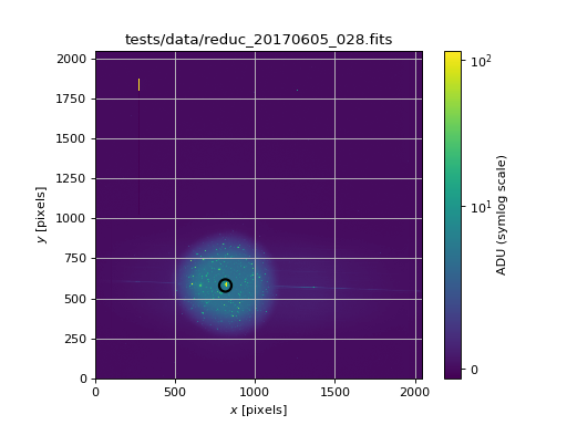
>>> from spectractor.extractor.images import Image
>>> from spectractor import parameters
>>> from spectractor.tools import plot_image_simple, plot_compass_simple
>>> f, ax = plt.subplots(1,1)
>>> im = Image('tests/data/reduc_20170605_028.fits', config="./config/ctio.ini")
>>> plot_image_simple(ax, im.data, scale="symlog", units="ADU", target_pixcoords=(750,700),
...                   title='tests/data/reduc_20170530_134.fits')
>>> plot_compass_simple(ax, im.parallactic_angle)
>>> if parameters.DISPLAY: plt.show()

spectractor.tools.plot_correlation_matrix_simple(ax, rho, axis_names=None, ipar=None, vmin=-1, vmax=1)[source]

spectractor.tools.plot_covariance_matrix(cov)[source]

spectractor.tools.plot_image_simple(ax, data, scale='lin', title='', units='Image units', cmap=None, mask=None, target_pixcoords=None, vmin=None, vmax=None, aspect=None, cax=None)[source]

Simple function to plot a spectrum with error bars and labels.

Parameters:

ax (Axes) – Axes instance to make the plot
data (array_like) – The image data 2D array.
scale (str) – Scaling of the image (choose between: lin, log or log10, symlog) (default: lin)
title (str) – Title of the image (default: “”)
units (str) – Units of the image to be written in the color bar label (default: “Image units”)
cmap (colormap) – Color map label (default: None)
mask (array_like) – Mask array (default: None)
target_pixcoords (array_like, optional) – 2D array giving the (x,y) coordinates of the targets on the image: add a scatter plot (default: None)
vmin (float) – Minimum value of the image (default: None)
vmax (float) – Maximum value of the image (default: None)
aspect (str) – Aspect keyword to be passed to imshow (default: None)
cax (Axes, optional) – Color bar axes if necessary (default: None).

Examples

>>> import matplotlib.pyplot as plt
>>> from spectractor.extractor.images import Image
>>> from spectractor import parameters
>>> from spectractor.tools import plot_image_simple
>>> f, ax = plt.subplots(1,1)
>>> im = Image('tests/data/reduc_20170605_028.fits', config="./config/ctio.ini")
>>> plot_image_simple(ax, im.data, scale="symlog", units="ADU", target_pixcoords=(815,580),
...                     title="tests/data/reduc_20170605_028.fits")
>>> if parameters.DISPLAY: plt.show()

(Source code)

spectractor.tools.plot_spectrum_simple(ax, lambdas, data, data_err=None, xlim=None, color='r', linestyle='none', lw=2, label='', title='', units='', marker='o')[source]

Simple function to plot a spectrum with error bars and labels.

Parameters:

ax (Axes) – Axes instance to make the plot.
lambdas (array) – The wavelengths array.
data (array) – The spectrum data array.
data_err (array, optional) – The spectrum uncertainty array (default: None).
xlim (list, optional) – List of minimum and maximum abscisses (default: None).
color (str, optional) – String for the color of the spectrum (default: ‘r’).
linestyle (str, optional) – String for the linestyle of the spectrum (default: ‘none’).
lw (int, optional) – Integer for line width (default: 2).
marker (str, optional) – Character for marker style (default: ‘o’).
label (str, optional) – String label for the plot legend (default: ‘’).
title (str, optional) – String label for the plot title (default: ‘’).
units (str, optional) – String label for the plot units (default: ‘’).

Examples

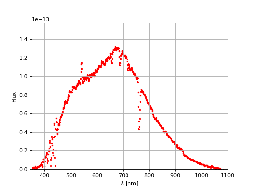
>>> import matplotlib.pyplot as plt
>>> from spectractor.extractor.spectrum import Spectrum
>>> from spectractor import parameters
>>> from spectractor.tools import plot_spectrum_simple
>>> f, ax = plt.subplots(1,1)
>>> s = Spectrum(file_name='tests/data/reduc_20170530_134_spectrum.fits')
>>> plot_spectrum_simple(ax, s.lambdas, s.data, data_err=s.err, xlim=None, color='r', label='test')
>>> if parameters.DISPLAY: plt.show()

(Source code)

spectractor.tools.plot_table_in_axis(ax, table)[source]

spectractor.tools.rebin(arr, new_shape, FLAG_MAKESUM=True)[source]

Rebin and reshape a numpy array.

Parameters:

arr (np.array) – Numpy array to be reshaped.
new_shape (array_like) – New shape of the array.

Returns:

arr_rebinned – Rebinned array.

Return type:

np.array

Examples

>>> a = 4 * np.ones((10, 10))
>>> b = rebin(a, (5, 5))
>>> b
array([[4., 4., 4., 4., 4.],
       [4., 4., 4., 4., 4.],
       [4., 4., 4., 4., 4.],
       [4., 4., 4., 4., 4.],
       [4., 4., 4., 4., 4.]])

spectractor.tools.rescale_x_from_legendre(x_norm, Xmin, Xmax)[source]

Rescale normalized array set between -1 and 1 for Legendre polynomial evaluation to normal array between Xmin and Xmax.

Parameters:

x_norm (np.ndarray)
Xmin (float)
Xmax (float)

Returns:

x

Return type:

np.ndarray

spectractor package

Subpackages

Submodules

spectractor.config module

spectractor.logbook module

spectractor.parameters module

spectractor.tools module

Module contents